RevTim

Aaaaah! That makes sense. Thank you!

I've just moved up to Affinity Photo 2, also purchased a couple of add-ons at the same time. All the default brushes and the new assets and brushes I've bought are locked (have a little chain icon next to them). I imported my old brushes and assets from v1. and they are all fine. Please can you tell me how to unlock them?

Even better! Thanks for the advice

I have a load of Photoshop shape files I've collected over the years and it always bugged me that there wasn't an easy way to import each .csh file into Affinity, especially now I have got rid of Photoshop all together. Fortunatley I saved all my PS plugins and shape files before uninstalling. I have just found a website which lets you upload the .csh files and then you can download each shape as a .svg vector image. It is then a slightly laborious process of open each vector svg file in Affinity and adding them to your Assets. Here's where you can upload your PS shape files: https://www.photoshopsupply.com/vector/csh-to-svg

Don't know whether this has been fixed on the latest version but I got around this by renaming "Acrylics" to "Paint Acrylics". The brushes are in alphabetical order which means that the any brush set with an lower alphabetical name than "Basic" will automatically be the deffault brush set. This could be useful as you could make your own brush set and call it (say) AABrushes, and it would be top of the last, therefore the default set.

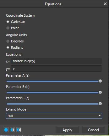
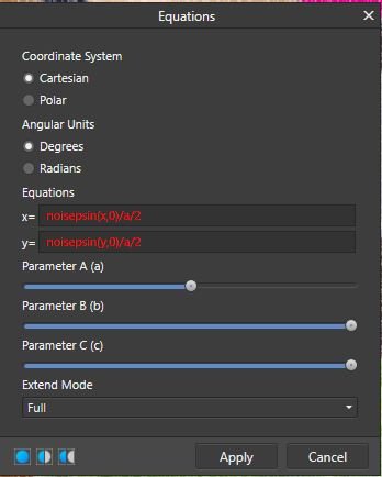
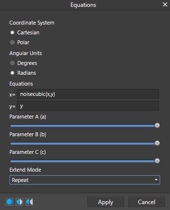
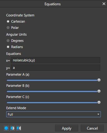
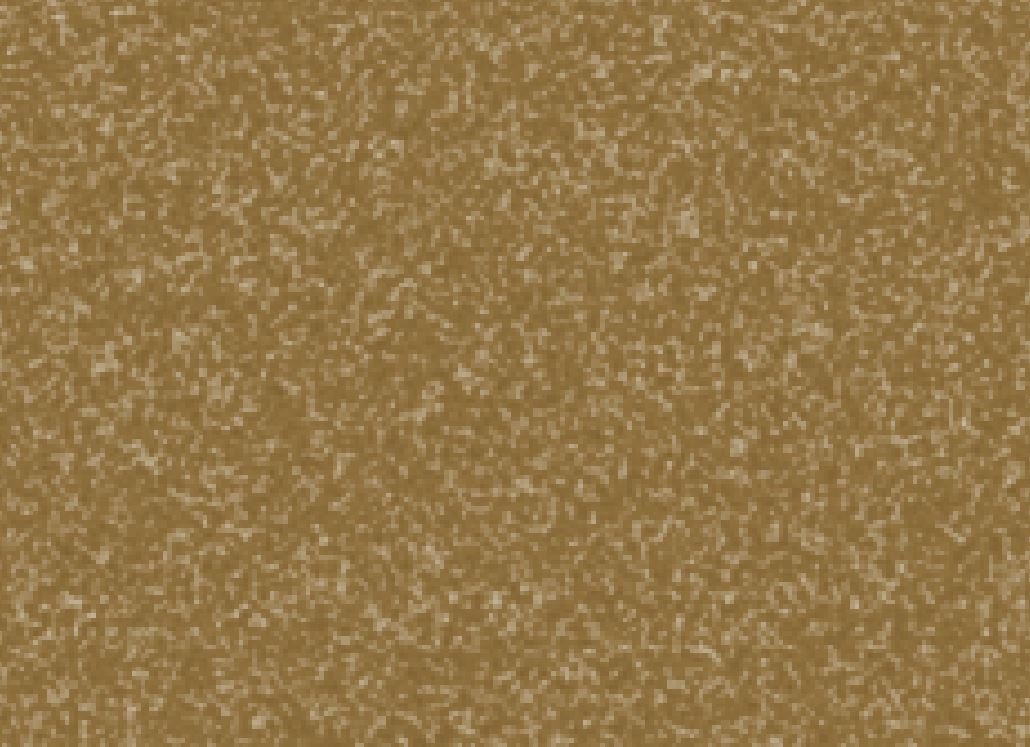
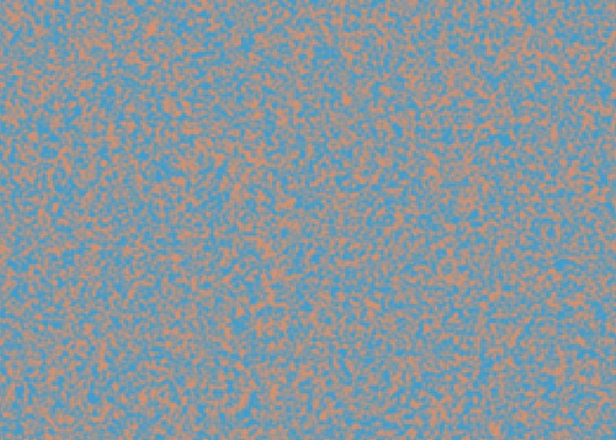
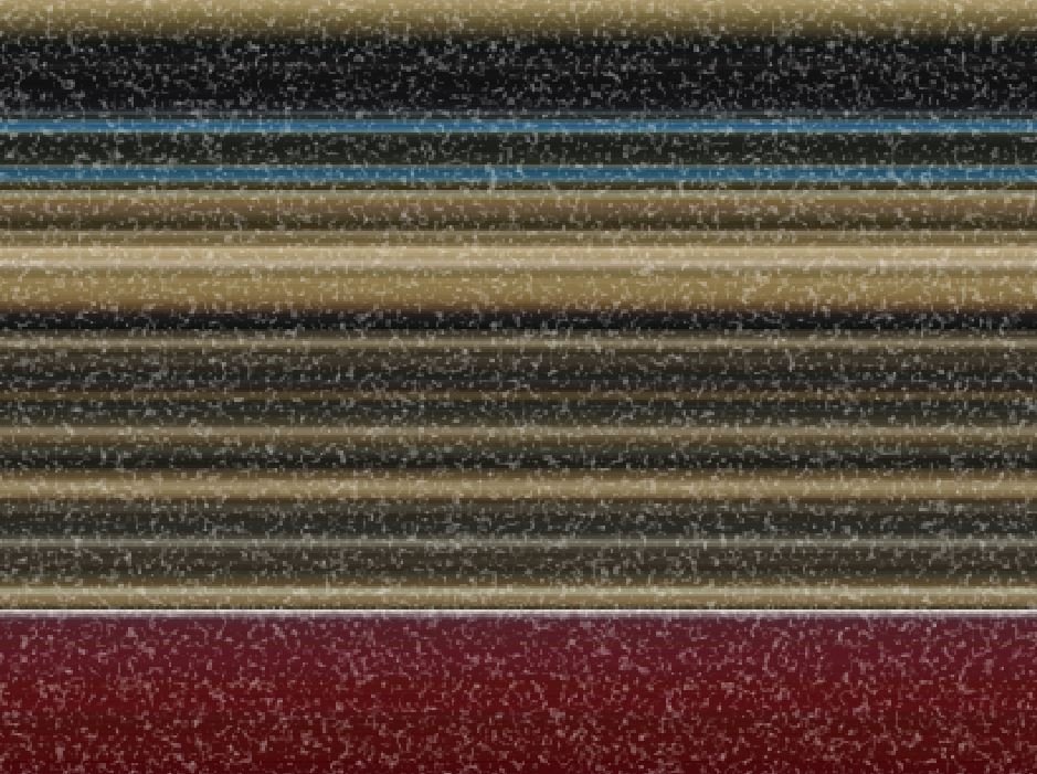
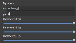
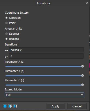
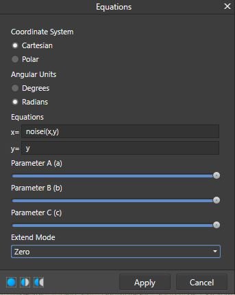
Part 1 of this tutorial which explains what procedural noise is and how it works can be read here. Introduction What follows are a few examples of how noise can be used practically and creatively. We will set up a couple macros to save for future use. If you aren’t familiar with macros, you can still follow the steps ignoring the macro parts. Alternatively, you can learn how to use macros on Affinity’s YouTube channel here. Before we launch into creating the macros, one, key discovery I’ve made which makes noise equations far more useful is that Equations noise can be generated on an empty pixel layer. Let’s do this now, so you can see what I’m talking about. Create a new, empty pixel layer above the background layer. Go to Filters Menu>Distort>Equations. Enter the basic noise Equation in the x= box – noise(x,y). Leave the default letter y in the y= box. Nothing happens! BUT… Change the Extend Mode to Full. Click Apply. Now you have a non-destructive noise layer of light “noise” type noise. If you want dark noise, just invert the layer. This layer can now be changed with layer blend modes (Overlay & Soft Light), rescaled, tinted, blurred, opacity reduced etc. Now we’ll create a couple of useful noise Macros. Add White Noise Macro Let’s use a different form of noise (noisecubic) to create a macro which will add white noise to images. First delete all layers apart from the background layer. Open the Macro tab and press the record button to start recording. Create a new pixel layer. Go to Filters Menu>Distort>Equations Apply the following equation: x= box - noisecubic(x,y) y= box - y Extend Mode - Full Click Apply. Change the noise layer’s name to White Noise. Press the stop button on the Macro tab. Save the macro as “Add White Cubic Noise” (without the quotes). Note: Hit the “Add White Cubic Noise” button a few times to see the effect increase or try changing the “White Noise” layer mode to Overlay or Soft Light. The effect of using the Add White Noise macro 3x Add Dark Cubic Noise Macro Follow all the steps for Add White Noise above but invert the White Noise Layer layer at the end and change the name of the noise layer to Dark Noise then save the macro. Controllable Weave Textures Early on in this tutorial we saw how putting the equation noise(x,1) in the x= box and a in the y= box generated vertical bars of averaged colour when applied directly to a photo pixel layer. If, instead, we apply the same equation to an empty pixel layer above a filled pixel layer, we have the foundation for creating a Weave texture (many textures, since there are so many types of noise). To create the macro, do the following: First delete all layers apart from the background layer. Open the Macro tab and press the record button to start recording. Create a new pixel layer. Go to Filters Menu>Distort>Equations Apply the following equation: x= box - noisepsin(x,0)/a/2 (note: 0 is the number zero, not the letter O) y= box - noisepsin(y,0)/a/2 Set the Parameter A to the midpoint. Set the Extend Mode to Full. Click Apply. Change the name of the layer to White Weave Texture. Save the macro as White Weave Texture. The Weave Texture – which shouldn’t work, since it’s all red – but it does! The weave texture equation explained: “noisepsin” is just the command to generate noisepsin type noise. (x,0) in the x= box tells Affinity to only make noise in the x direction (left to right, I think) (y,0) in the y= box tells Affinity to only make noise in the y direction (top to bottom, I think In both boxes the 0 (number zero), I suspect, is the amount of offset from the starting point in the top left-hand corner. Certainly all changing this number does is change the pattern ever so slightly. /a – The / sign means “divide by”; the letter a activated the Parameter A slider. /2 means “divide by 2”. Purely by experiment I found that multiplying the equation by a (noisepsin(x,0)*a) made the Parameter A slider have the effect of gradually filling the transparent areas of the texture with white when the slider was moved to the left. Dividing by 2 (noisepsin(x,0)/a), on the hand, had the effect of make the Parameter A slider gradually reduce the number of stripes as the slider was moved to the left. Dividing everything by 2 (/2) at the end meant that the default position of the equation is now half-way along the Parameter A slider. Moving the Parameter A slider left gradually decreases the amount weave; moving it right increases the amount of weave. So, the whole equation instructs Affinity to generate noisepsin noise, from left to right, and from top to bottom separately (creating vertical and horizontal stripes), but the amount of noise is going to be controlled by the Parameter A slider. Weave Texture applied to the test image – the layer mode was set to Overlay. Adjustable Gradient Background from any Image This macro will generate adjustable gradients from any image. To create the macro, do the following: First delete all layers apart from the background layer. Open the Macro tab and press the record button to start recording. Duplicate the layer with Ctrl+J. Go to Filters Menu>Distort>Equations Apply the following equation: x= box - noisecubic(x,y) y= box – y Extend Mode – Repeat Click Apply. Go to Layer menu>New Live Filter Layer>Blur>Gaussian Blur IMPORTANT: Make sure you put a tick in the Preserve Alpha box, or the blur will not go to the edge. Set the Radius to 50px. Close the Live Gaussian Blur Dialogue (Don’t Merge, Delete or Reset). Select the Gaussian Blur’s parent layer (should be the top layer). Rename this layer as Gradient Blur. Press stop on the Macro recording tab. Save the Macro as Horizontal Gradient from Image. When you run the macro on any photo or image (must be a pixel layer, don’t forget), it will generate a horizontal gradient with a live blur which you can adjust. Gradient produced from the test image with Gaussian Blur set to 100px See if you can create a macro which will generate a vertical gradient. Adjustable Coloured Noise This macro creates a layer of coloured where you can choose any colour at any brightness or saturation level. It uses the same steps as the horizontal gradient macro, but with a few tweaks. To create the macro, do the following: First delete all layers apart from the background layer. Open the Macro tab and press the record button to start recording. Duplicate the layer with Ctrl+J. Go to Filters Menu>Distort>Equations Apply the following equation: x= box - noisecubic(x,y) y= box – a Extend Mode – Full Click Apply. Add a new HSL Adjustment Layer. Close the HSL Adjustment Layer Dialogue (Don’t Merge, Delete or Reset). Select the layer beneath the Adjustment Layer (choosing “Select 1 layer below current”) Rename this layer as Coloured Noise. Save the Macro as Coloured Noise. To use the macro, run it, then drag the HSL adjustment layer onto the Coloured Noise layer. You will then be able to adjust the coloured noise without affecting layers underneath (double-click on the HSL layer icon). Conclusion I hope I’ve show that using noise in the Equations filter is: a.) less scary than you thought, and b.) genuinely useful, with many potential applications. Note to Affinity developers – It would be sooooo helpful if the next release of Affinity had the ability to save Equations as presets in the same way as the Procedural Textures filter. That would save having to use macros and make them even more practicable.

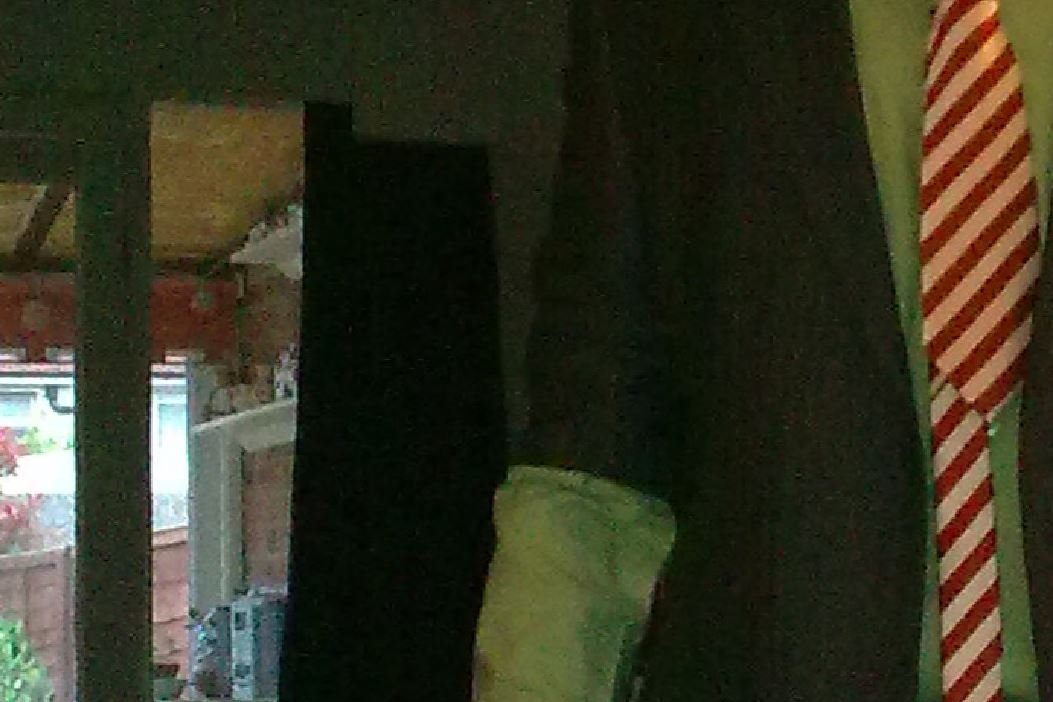
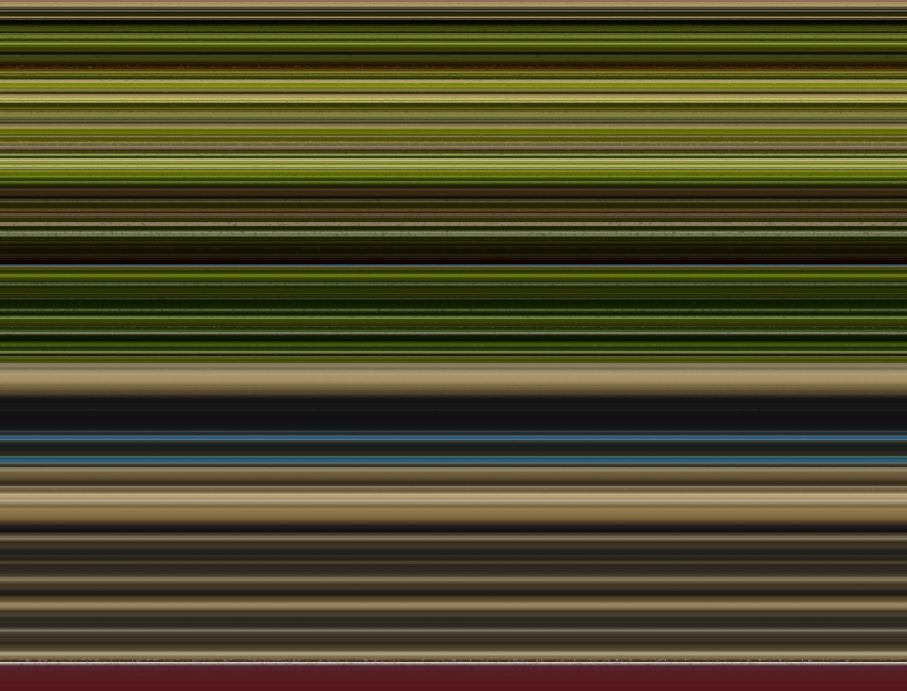
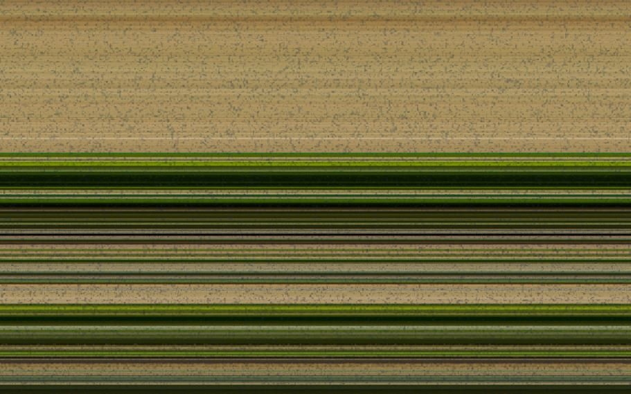
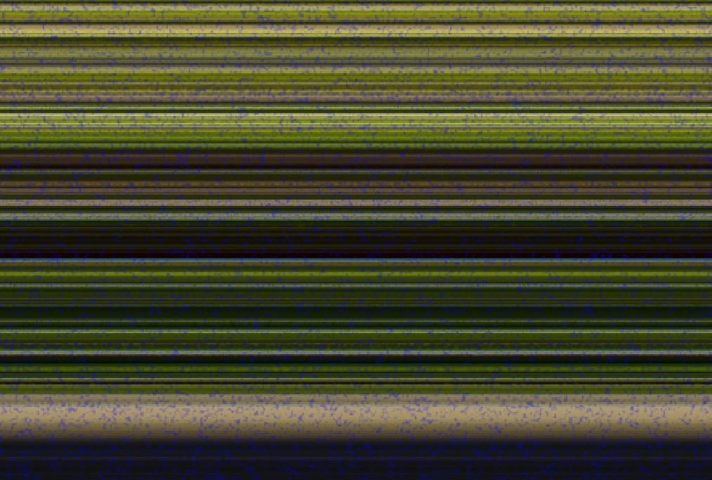
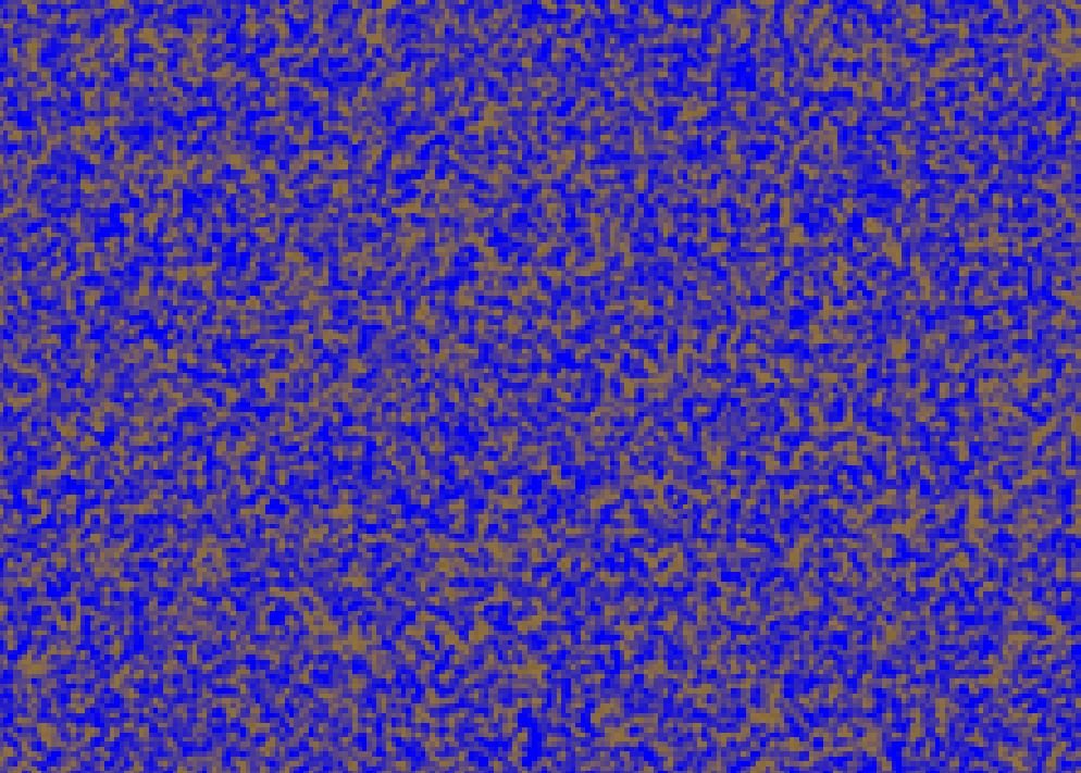
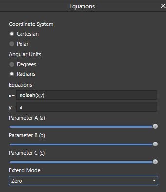
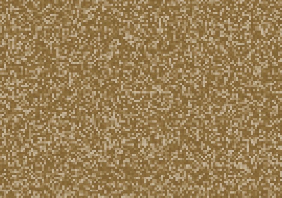
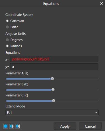
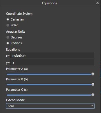
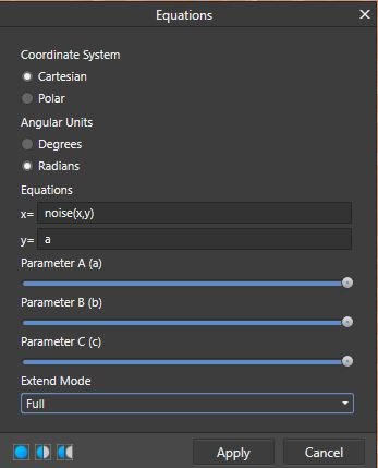
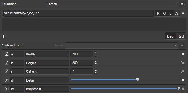
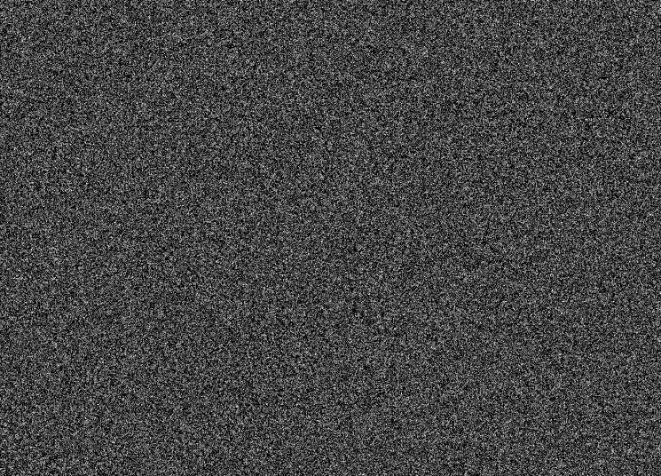
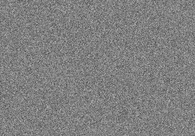
Summary This tutorial: Is aimed users with little or no knowledge of the Equations filter. Explores what “noise” is, in the Affinity Photo filters – particularly how it appears in the Equation filter. What the effects of “Extend Modes” have on noise generated in the Equations filter. What the effects are of using the “a”, “y” or other equations in “y=” part of the Equations. Shows how noise equations can be used effectively on an empty pixel layer. Offers some practical uses for noise equations with macros. Introduction The aim of this tutorial is to explore the inner workings of the “noise” command as it’s used in the Equations filter in a practical and experimental way. I am not a computer programmer or a mathematician – so this is layman’s perspective, not a technical tutorial. The goal is to help users who have only a rudimentary understanding of the Equations filter get to grips with and find uses for the noise function in the Equations filter. Hopefully, any inaccuracies will be picked up by other users in comments. I’d like to thank John Rostron, whose more technical article about the noise function made me curious – you can read it on the forum HERE. Preparation If you want to follow in Affinity Photo the experiments I’ll make in this article, you’ll need to do the following: Open a test image or download mine – link at the bottom of the article. Make sure the image is a pixel layer not an image layer. If it says “Image” on the layer in the layer palette, right-click and select “rasterise…”. Duplicate this layer with Ctrl+J. Create a new pixel layer above the bottom Background layer and fill with a blue colour (eg. R:0, G:0,B250). This will enable you to see any transparent areas made by noise in the top layer. Noise vs Procedural Noise So, what is “Procedural Noise”? In digital imagery like digital photos and scanned images, noise is unwanted artifacts in the form of random variations in the colour and tone of pixels in an image, which are not part of the original image. They are generally produced as a result of electronic interference. If you push the ISO on your digital camera to its highest rating and take a photo in low light, zoom in and you will likely see spots, speckles and coloured patches which were not a part of the scene (see image below). A noisy image produced on a high ISO on an older camera. Usually (and mainly in photography) this noise is unwanted, but it can be used creatively for special effects or for artistic purposes by graphic designers and artists, so software like Affinity Photo usually provides effects filters which let the user add various forms of noise to their images. This noise is produced by a mathematical algorithm or piece of computer code, and so is made by a procedure – hence “Procedural Noise”. Here are couple of examples of procedural noise used artistically: In the image above, I used the Filters>Noise>Perlin Noise filter in combination with the Displace Filter for a quick artistic effect on the right-hand side – the left side is the original image. Both the background and the text textures in the image below were created using noise equations in the Equations filter. Affinity Photo provides the user with four main ways to introduce noise, all found in the Filters menu. Add Noise… and Perlin Noise… are found in the Noise section of the Filters menu. These are the simplest way to add noise, since they have a user-friendly interface. Noise can also be introduced through the Procedural Texture and Equations filters found in the Colours and Distort sub-menus. Both these require the user to enter equations, which can make them seem daunting, if not a no-go area, as there virtually no guidance on how to use them in the help file for those without any technical knowledge. If you want to begin understanding and using Procedural Textures in an accessible way, try my absolute beginner’s tutorials here – which also uses noise functions. Procedural Textures – Key Features The single most important/useful thing about procedurally produced noise is that it can be produced at any scale or resolution of image without degradation. Because it is a random pattern (pseudo-random, if we’re being pedantic) produced by an equation, the pixels it produces are not fixed or ‘real’ until the apply button is clicked. Instead, like vector graphics, the work at all sizes and scales of image. You can fill a 1mp or 100mp image with noise and the pattern will never repeat or degrade. One feature I have discovered, which is often overlooked, is that procedural noise is composed essentially of two areas: areas with the noise pattern and the areas between, which I am calling negative space. It turns out, the negative areas are just as important as the bits of noise, as we’ll see later. More precisely, it seems that there are parts (pixels, ultimately) which are solid colour, and others which are increasingly transparent – which become more evident when using noise in the Equations filter. Let’s take a look at very basic noise in the Equations Filter: Check to make sure the top layer of the test image is still selected. Open the Equations filter dialogue by going to Filters>Distort>Equations. Enter the following equation exactly as it is in the with no capitals or spaces: In the x= box type noise(x,y) In the y=box type the letter a (Which I’ll explain later). From the Extend Mode list, select Full. Coordinate System should be Cartesian, and Angular Units should be Degrees, by default – from now on everywhere I describe inputting an equation in the Equations dialogue the default settings of Cartesian and Degrees will be assumed. DON’T click apply, leave the dialogue open so you can follow the experiments below. To see the noise more clearly, hold down Ctrl and scroll your mouse wheel forward to zoom in. You can now see clumpy, fuzzy blobs of solid colour with fuzzy white patches of negative space. Zoomed out, it’s the coloured bits that we perceive as noise. I’ll explain the reason for the strange colour in a moment. What’s going on? What’s really happening is that the noise command generates random vertical and horizontal bars of tone shaded from white to a solid colour. We can see this by changing the equation. At the moment noise(x,y) is an instruction to make noise in the x and y directions - horizontally and vertically. Change the equation so that it reads noise(x,1). You should see random vertical bars in various tones of colour like this. Now change the x in the equation to a y, so the equation reads noise(y,1). You should see random horizontal bars in various tones of colour like this. This indicates that noise(x,y) is really a blend of the two. What the deal with the colour? When the noise(x,y) equation is used in combination with the Full noise Extend Mode, the filter generate noise which is a kind of average colour of the whole image, though this is not exactly the same colour as would be produced by the Blur Average filter. From my experiments, these white areas are, in reality, appear to be areas of transparent and semi-transparent pixels, depending upon the tone of the pixels. Pixels of the true averaged colour are opaque whilst lighter tones are increasingly transparent, until you get to white which is entirely transparent. At the moment, we are seeing the light pixels as white because, in this instance, the Extend Mode we’re using is Full, which makes the white areas opaque. I’ll explain a bit more about transparency later, when we look at other Extend Modes. There’s more than one kind of noise! Until now, I’ve been using the word “noise” to talk about procedural noise in general terms. In fact, in the Equations Filter the word “noise” is the name of just one particular type of noise. In the programming language used to generate procedural noise in both Procedural Textures and Equations, there are dozens of different types of noise (noise, noisei, noiseh, noisecubic, noisesin etc.), each producing a slightly different type of noise. The differences are, perhaps, more noticeable in Procedural Textures where you can magnify them to create interesting patterns, effects. You can see the full list if you look up Procedural Texture in the help file. Scroll down the page and you’ll eventually come to the lists of different noise types. For a very different kind of noise add the letter “i” after the word noise, so the equation reads noisei(x,y) in the x= box (till with a in the y= box and the Full Extend Mode). This makes noisei type noise, which is blocky and pixelated. noisei type noise Now try substituting the letter “i” with an “h”, so you have noiseh(y,x) in the equations. You should end up with something like this: noiseh type noise You can now clearly see the coloured fuzzy blobs of noise with the negative white areas between. Extend Modes make a MASSIVE difference Let’s prove that white areas and lighter tones are, in fact, areas of transparency. Just to remind you, Extend Mode is last option at the bottom of the Equations filter dialogue. It contains a drop-down list with Zero, Full, Repeat, Wrap and Mirror. Each mode has a different effect upon what the equation does to the image. Change the Extend Mode to Zero. noiseh(y,x) with Zero Extend Mode. Suddenly, you can see the underlying image (the blue layer) through a veil of noise. Experimenting with different extend modes To experiment with different Extend Modes, we’ll use the first noise equation we started with. It should still be open, but if it isn't, set it up the Equations dialogue as follows: That letter a in the y= box essentially activates the Parameter A slider, turning it into a sliding controller. I’ll come back to this later. Try testing out the Equations with different Extend Modes, at the same time as sliding the Parameter A slider back and forth. Here’s what I observed. Zero Extend Mode produces noise with transparent negative areas revealing the layer underneath the current layer. The noise pixels are made more transparent by sliding the Parameter A slider to the left. There is an initial brightening of the noise before it begins to fade, never quite going completely transparent. Full Extend Mode fills the layer with white overlain with noise. The noise pixels are made more transparent by sliding the Parameter A slider to the left. Repeat Extend Mode produces sparse noise (with this image) on a solid field of averaged colour. Moving the Parameter A make the noise and background colour lighter. Note: in one image, I found that the Repeat Extend Mode filled the layer with averaged colour and zero noise. Wrap Extend Mode is unpredictable from images to image. In the image, it averaged colour noise on a background which is the inverse colour of the noise. Moving the Parameter A to the left changes the relationship of the positive and negative colours, intensifying the background colour whilst making the noise more transparent. Mirror Extend Mode, gives identical results to Repeat, in these experiments. Dealing with the “y=” box So far, we have only had the letter a in the y= box. That is because the the y= equation box cannot be left blank. It must contain a value of some kind; either a letter*, a number, or another equation (which I’ll come back to later). If you enter the letters a,b or c in the y boxes then the A,B or C parameter sliders become active, giving customisable control of Equation depending upon which extend mode you use. *note: only letters that have a function in the Equations filter produce a result when used alone in x= or y= boxes. I will list other useable letters at the end of the article. However, if you leave the default letter “y” in the y equation field, you get completely different results with different Extend Modes. Try the following tests using noisei(x,y) in the x= field and y in the y= field. You’ll need to zoom out at little to get an idea of what is happening (hold down Ctrl and scroll the mouse wheel backwards). You should see something like this. Zero extend mode (above) produces random horizontal bands of colours which are averages of the area the bands cover. The negative, transparent and semi-trasparent areas of the noise pattern punch holes through the current layer revealing the layer underneath. Full extend mode (above) produces random horizontal bands of colours which are averages of the area the bands cover. The negative, transparent and semi_transparent areas of the noise pattern are white instead of transparent. You need to zoom in to see this more clearly. Repeat and Mirror, both produce random horizontal bands of colours which are averages of the area the bands cover with little or no noise. The Wrap Extend mode (above) is a weird one. It creates the same horizontal bands of colour, but this time, the negative spaces are of varying colour, perhaps inverse complimentaries? Using noise equations in both x= and y= boxes Adding a noise equation to the y= box in addition to the one in the x= box has the effect of adding a second layer of noise to the image. The resulting noise is now similar to the earlier noise where we put an a in the y= box. If the y= box contains the same equation as the x= then the effect, though, appears to be to increase the contrast between noise and negative areas. However, if equation in the x= box is noise(x,y) and the y= box is noise(y,x), the effect is to increase the overall amount of negative/transparent/white areas. What this means is that you can overlay two different kinds of noise, if you wish. Try for example, using noiseh(x,y) in the x= box and noiseh(y,x) in the y= box. This concludes Part 1 of the tutorial. Part looks at putting all to use with some practical examples. Scroll down for the link to Part 2. Notes Useable letters which can be use in the x= and y= boxes a, b & c – activate the parameter sliders in the dialogue h produces light, near neutral noise - Try h+a and h*a in the y= box with various modes. x & y Noises with the letter “h” in their name like (noiseh, noisehpsin, noisehcubic etc.) create harmonic noise, which has greater negative areas. Special note re. Perlin Noise Perlin noise, which you may have come across in the list of noise types, is a particular type of noise invented by Ken Perlin, who was looking for a way to generate more natural/realistic looking 3D textures. It has a more “clumpy” look to it. When it is scaled in 2D imaging software like Affinity it can create wonderfully versatile natural-looking textures from clouds to hair and even wood grain. Sorry to say, I have yet worked out how to scale any noise in Equations. Nevertheless is still a useful variation of noise. The Perlin noise command requires four pieces of information to work properly. I don’t want to go into any kind of technical depth here, so just try the example below (note the position of the Parameter A, B, and C sliders): Explanation: Perlinsin – a type of Perlin noise. rx,ry – generates the noise. The r before x and y means you can click in the image and drag the noise around. a*10 – Activates the Parameter A slider which seems to control softness and brightness b – Activates the Parameter B slider, which seems to control softness and graininess. /c/2 _ Activates the Parameter B slider, which acts as a sort of contrast control, change the spread of midtone pixels. GO TO PART 2

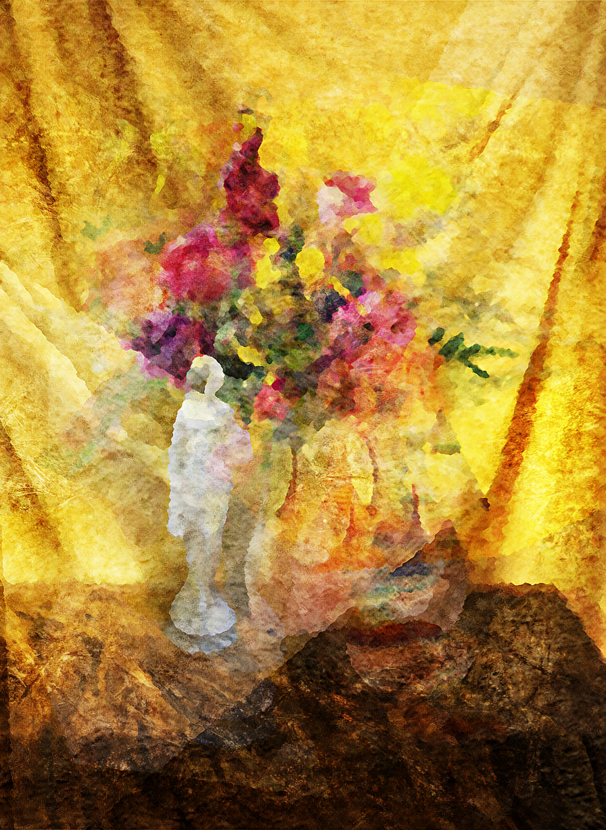
Wow! Thanks for the very flattering comparison. If only my work was a groundbreaking as Welle's film! I was going for semi-abstract in style, although I also like doing completely abstract work - which may be my next project.

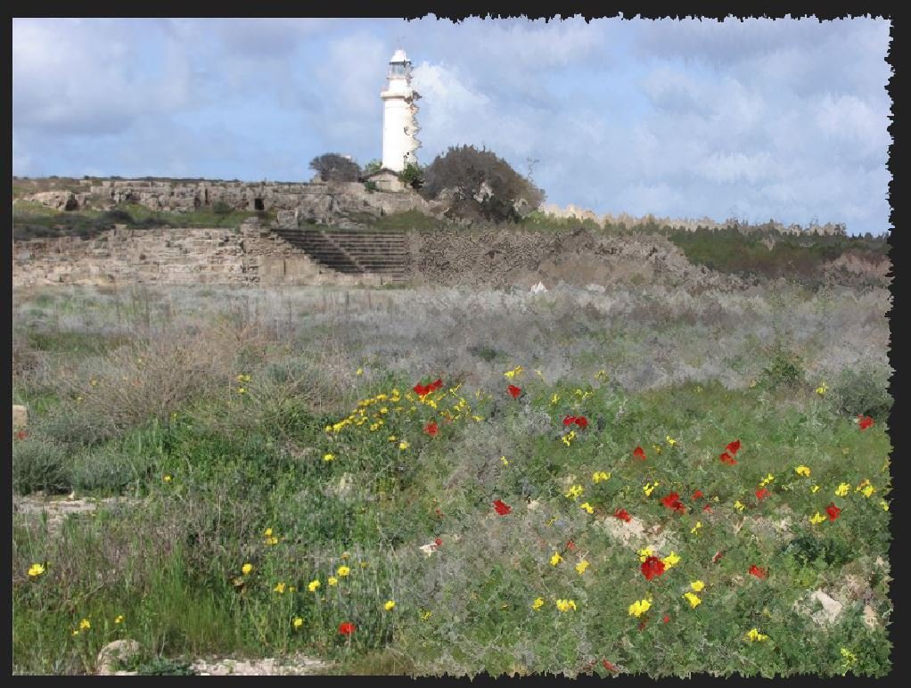
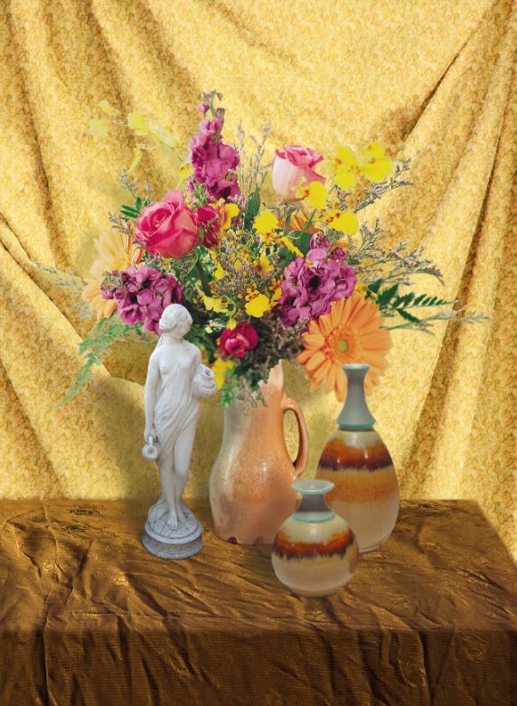
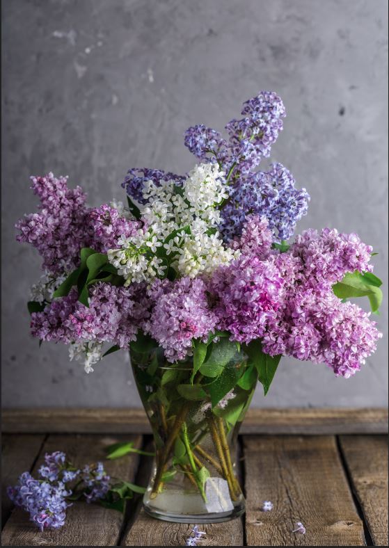
I love to see how far I go with creating a painterly look beginning with a photo. The original photo (below) is actually a montage of many images found on the web - vases, flowers, draperies, figurines, etc. were are separate images. The resulting combined painting was created solely from Affinity Photo's default filters & layer blend modes, and without using any brushwork. Ultimately, the document contained 22 layers. Original Photo/montage

It's a brilliant workaround. I found that by default my Canon scanner is set to idiot mode - automatically choosing jpeg, standard quality and sent to Documents(?!?!?), but once I went deeper into the settings I found I was able to set what I wanted to do with the scanned image. On my Canon TS6050 scanner I had to select the Scangear option, instead of selecting "Photo". That allowed me to change to TIFF or no compression jpeg and then send to Affinity Photo. In the Scangear I had to first add Affinity Photo as an Open With program (In my Windows 10 Affinity Photo exe is in Programs, not Programs 86. I also had to make sure that checked Preview so I could see what was being scanned. However, having done all that, I'm pretty much back to where I was with Photoshop ☺, the main difference is that I have to choose where I want to save the 'document' before the image opens in Affinity. So long as I set that to Desktop, I can then work away in Affinity, save the result wherever I want and then delete the desktop file when I'm done. It's not quite as smooth as going straight into Affinity, but it works. I believe the phrase 'happy bunny'. Thanks John.

Neverthless I CAN scan directly into PS Cs3 on my 64 bit system. It may not be a 64bit image, but it's the workflow that's important. The twain scanner driver and software PS uses are better than the very basic Canon scanning utility in Windows.

On PC. No Acquire Image in the File Menu. The help says to scanning is not supported. "For Windows, Affinity Photo does not offer scanning directly from within the app. We recommend using your own scanner's software to acquire image."

Please would you add the ability to scan straight into Affinity Photo in the next release?

I have a document in Affinity Photo with multiple layers each of which is intended to be a separate page in a PDF which I export. (So, layer1, would be page 1, layer2, page 2 etc.) I haven't been able to find out how to do this yet as I haven't been able to find an option for exporting layers as separate pages in a single PDF document. Is there a way to do this, please?

I love to see how much of a painterly look I can get from photos using just Affinity's standard filters. I created this impressionistic oil painting of lilacs in a vase from a stock photo I found in the Pixabay section on Affinity Photo's Stock tab (Thanks to Daria Yakovleva for contributing her photo, which you can see below). There is no brushwork involved in this; it's all filters, layer blend modes and adjustment layers along with a few textures I also found in the stock imagery. Here's the original photo: (Photo by Daria Yakovleva from Pixabay)

Ooooooh, doh! This is why I don't earn the smart money ☺. Yeah, once I've got the navigation set to 100% it previews fine. Shame it doesn't preview accurately when viewing the whole image, though. Thanks. Tim

The Zoom level is 100% - fully zoomed out. I think the problem is more pronounced when 'circular' is checked. It also seems to depend on the content. Experimenting with other photographs I find that the preview/apply difference is less pronounced in some images.

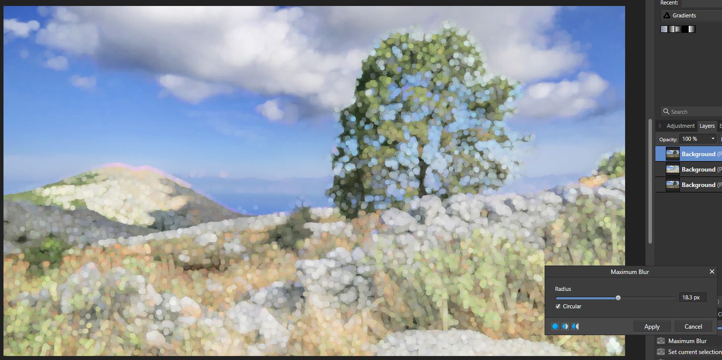
The previews for both Minumum and Maximum Blur do not show the correct result after you hit apply. Minimum Blur goes significantly darker after applying and Maximum Blur goes much lighter (producing a halo the more blur is applied.) See xamples attached.

That's nicely done, John and thanks, as always, for the editorial notes. With regard to the issues you had with tutorial: Sub-presets are in the main PT dialogue. They are found by clicking on the presets drop-don list in the BOTTOM custom Inputs section. They are also renamed and deleted from here rather than the Preset Manager. To rename a layer whilst making a macro, click on the layer's name in the layer palette (for some reason you can't get the rename layer option by right-clicking on the layer or in the Layer menu). The problem I had with editing my posts has been fixed by the Affinity Team, so I have eidted the tutorial to try to make these issues clearer.

I still can't edit my older posts. I can happily edit my most recent posts, but I'm not getting "author" by my earlier ones. Frustrating!

"Pre-pain" macro😅 I wonder what a post-pain macro feels like. Honestly, I'm hopeless at spotting my own typos. I wrote a book about Christian spirituality. In it I quote Psalm 156 - Psalms only goes up to Psalm 150. And in a church magazine I was trying to quote a line from a Christmas carol which goes "... One is for God's people, in every age and day." Just before I hit "Print" I noticed I'd typed "One is for God's poodle." Just as well I spotted it, who knows, maybe he's a cat-person! Thanks for picking up those. Tim

I'm sorry I've only just gor back to you. What a great tips! Thanks for those. The Fade command isn't anything to do with layer opacity. After you have applied a filter, you go to the Layer menu and the top item will be "Fade (filter name)". You can then Fade the filter by any amount. I'm sorry for the confusion. I should have made it clear that when I say Layer> or Edit> I mean click on those menus as in Edit>Fill with primary colour, or Filters>Blur>etc.

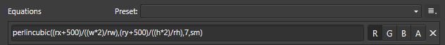
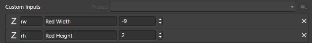
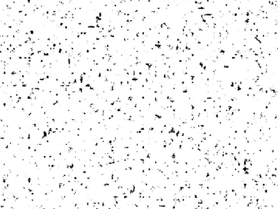
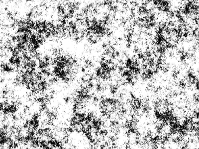
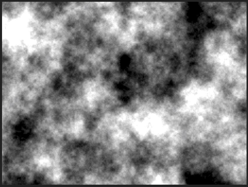
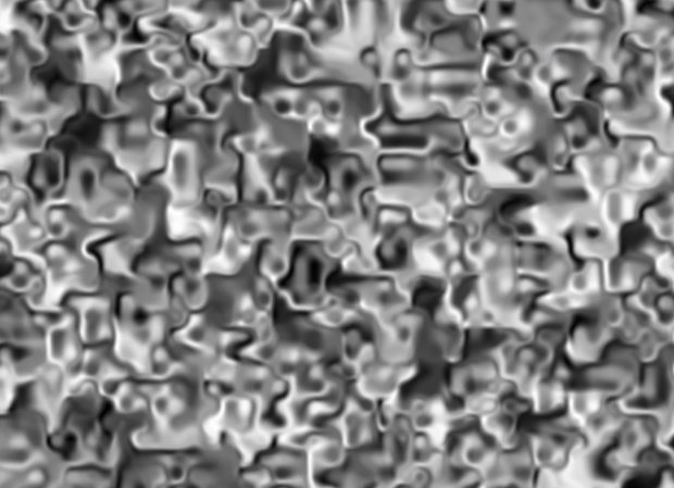
USING BRACKETS IN EQUATIONS PART 2. (Part 1 is HERE.) In the tutorial we are going to look at a more complex example of using brackets to expand the usefulness of Procedural Textures. Using the techniques we’ve learned so far, we’ll produce a beautiful and adjustable watercolour background texture like this: Super-Tweaking! First, create a new document with a filled pixel layer and add a Procedural Texture. I you are unsure how to do this, look at the beginning of the previous tutorial. Select the Simple Perlin Noise preset. To create the watercolour background texture I showed you at the beginning of this tutorial, I started with the basic Simple Perlin Noise preset equation - perlinsc(rx/200,ry/200,7,0.6)*0.7. At face value, it doesn’t seem to bear any relation to perlincubic((rx+500)/((w*2)/b),(ry+500)/((h*2)/c),7,a), which was my kicking-off point for making the texture, but let’s break it down: Important note: This equation is going to be used for the red channel only. We’ll need to two more for the green and blue channels. Don’t add them now. I’ll take you through the assembly of the texture later. Instead of making perlinsc I thought I’d experiment with another Perlin noise function – I picked perlincubic (there is a full list of Perlin noise types in the help file under Procedural Texture). The whole set of instructions for making perlincubic noise are contained (must be contained) within an opening and closing set of brackets: perlincubic((rx+500)/((w*2)/b),(ry+500)/((h*2)/c),7,a) NOTE: There’s no brightness control at the end outside the closing bracket – I ditched it for the sake of simplicity. Looking back at the perlinsc equation, it has FOUR parts, each separated by commas. perlinsc(rx/200,ry/200,7,0.6) It’s the same here: perlincubic((rx+500)/((w*2)/b),(ry+500)/((h*2)/c),7,a) The four sections are: SECTION 1 - ((rx+500)/((w*2)/b) This segment is the instruction for how to make noise across the image. It is has got three parts (rx+500), (w*2), and b. Each part is separated by a / (divide) symbol. rx we know from the earlier tutorials is an instruction to make click-draggable noise across the screen starting in the top left corner. +500 is a way of telling Affinity to make the starting point for the texture 500 pixels in. This is must be enclosed in brackets so that Affinity knows to read this as a single instruction. It is now going to DIVIDE that by the next part (w*2). w is C++ code for the width (I think) of your document, which in this instance is to be multiplied by 2. In order to just multiply the width by 2 and nothing else, the w*2 must also be put in brackets – (w*2). Using the width of the document to determine how the texture is made appears in some of the default equations like Urban Camoflage. Purely by experimentation with other equations I discovered that dividing rx and ry by the width and height is a good way offsetting the texture at the same time as scaling them. The b segment of this section is a custom input. Affinity looks at all the stuff in front of the b and then divides it by whatever number is put in the b Custom Input controller. Look, as a texture tweaker, it’s not essential to understand the maths, just what the equation is doing. It’s taking all sections enclosed by brackets as separate parts to be dealt with individually. So long as you keep the stuff inside the brackets you can tweak and experiment to see what happens. Numbers inside brackets can be swapped for Custom Inputs and vice-versa, multiplication signs can be swapped for division signs etc. Just remember the brackets golden rule – What happens in brackets stay in brackets. SECTION 2 - (ry+500)/((h*2)/c) Is the next section of the equation does exactly the same, but instructs Affinity to make the noise going down the image. h is C++ code for the height of the document and c is another Custom Input. SECTION 3 - 7 This section is an instruction to set the amount of detail or noisiness (officially called Octaves). SECTION 4 - a This segment controls the smoothness of the detail (officially called Persistence). Creating the Texture Open the Procedural Texture dialogue box, if you haven’t already opened it (Filters>Colours>Procedural Texture). If there are any equations in the top section, delete them clicking the X at the end of each line. Likewise, if there are any custom inputs in the bottom section, delete those in the same way. Click the + sign at the bottom of the Equations section three times to add three empty equations lines. Each should have the R, G, & B, highlighted in turn. Add 6 Z custom input number controllers and one -1,1 custom input sliding controller. Copy and paste this equation into the Red channel equation box: perlincubic((rx+500)/((w*2)/b),(ry+500)/((h*2)/c),7,a) To make the equations a little easier to make sense of, change the b to rw (for Red Width); change the c for rh (Red Height); and change the a at the end of the equation to sm (smoothnes). The only reason for doing this is for ease of working - sm doesn't do anything, you could just as easily type banana. Stick with sm for now so that the equation now reads: perlincubic((rx+500)/((w*2)/b),(ry+500)/((h*2)/c),7,sm) Nothing will happen until we assign the custom controllers with the same values. First, we’ll set the smoothness, that way we’ll see the texture develop as we edit the other controls. Change the letter g in the -1,1 input to sm, name it Smoothness, and set the slider to about 25%. Change the first Z input value (a) to rw. Give it the name, Red Width. Give it a starting value of -9. Change the second Z input value (b) to rh. Give it the name, Red Height. Give it a starting value of 2. opy the equation from the Red channel equation line and paste it into the Green channel equation line. This time change rw, and rh to gw and gh. Change the next two Z custom inputs to match the changes, creating controls for Green Width and Green Height. Set the width amount to 12 and the height to 2. Copy the equation a third time, pasting it into the Blue channel equation line. Change the equation again to be bw & bh. Change the last two Z controllers (e & f) to bw & bh, naming them Blue Width and Blue Height. Set the Blue Width amount to 16 and the Blue Height amount to 3. The final texture dialogue should look like this: Save this preset as Watercolour Background. If you find at any stage you’ve got a blank document, you may have a mismatch between the value names in the equation and value names in the controls. I find it’s very easy to change rw (red width) to rg instead of gw, for instance. You’re probably wondering why I used a -1,1 slider instead of a 0,1 slider. The main reason is that you can get different pattern variation either side of the mid (0) point. Variations Don’t forget this is click-draggable! Colourful Clouds Red Width = 3 Red Height = 2 Green Width = 4 Green Height = 3 Blue Width = 7 Blue Height = 5 Slider 20% Horizontal Rainbow Bands Red Width = 3 Red Height = 151 Green Width = 5 Green Height = 157 Blue Width = 7 Blue Height = 159 Slider 30% This Last one looks great on text: FINAL TIP: Texture not working? Count your brackets and keep your commas! When you have an equation with lots of nested sets of brackets (e.g. (((a*b)*(c*d))*2), it’s easy to miss adding an opening or closing bracket. If you end up with no texture, count the number of opening brackets (, and then count the number of closing brackets ). They have to be the same. If they aren’t, you’ve missed one or added an extra one. Finding the error can be tricky. First look to see if the individual parts are contained in brackets e.g. does a*b have both opening and closing brackets. If that doesn’t work, try working from the outside in – start with the outermost pair of brackets and gradually work inwards. When tweaking existing equations, it is also easy to accidentally delete a comma, particularly with long equations in which you have added lots of extra values and expressions.

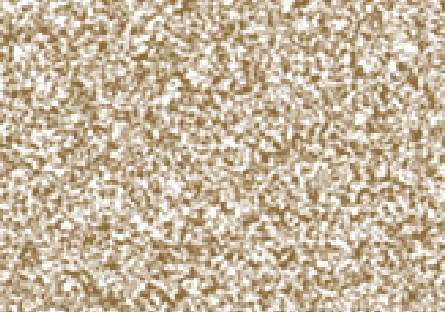
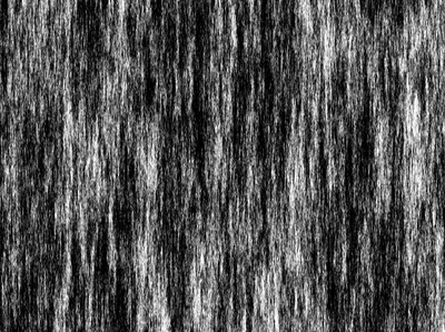
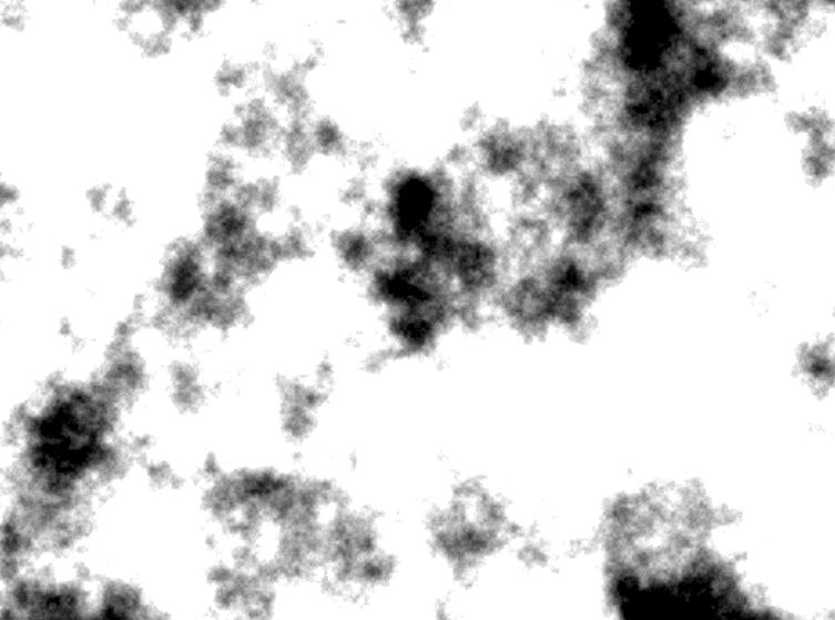
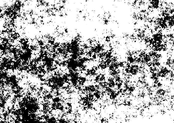
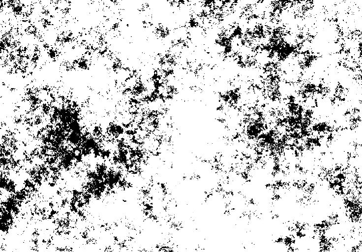
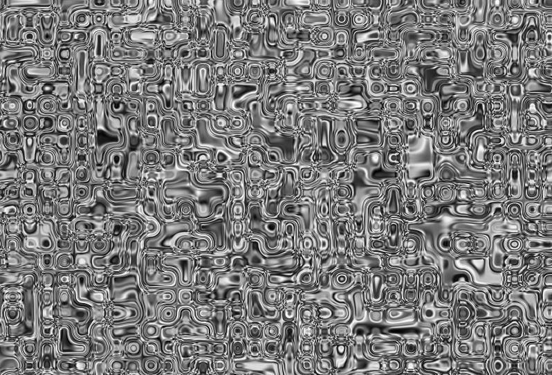
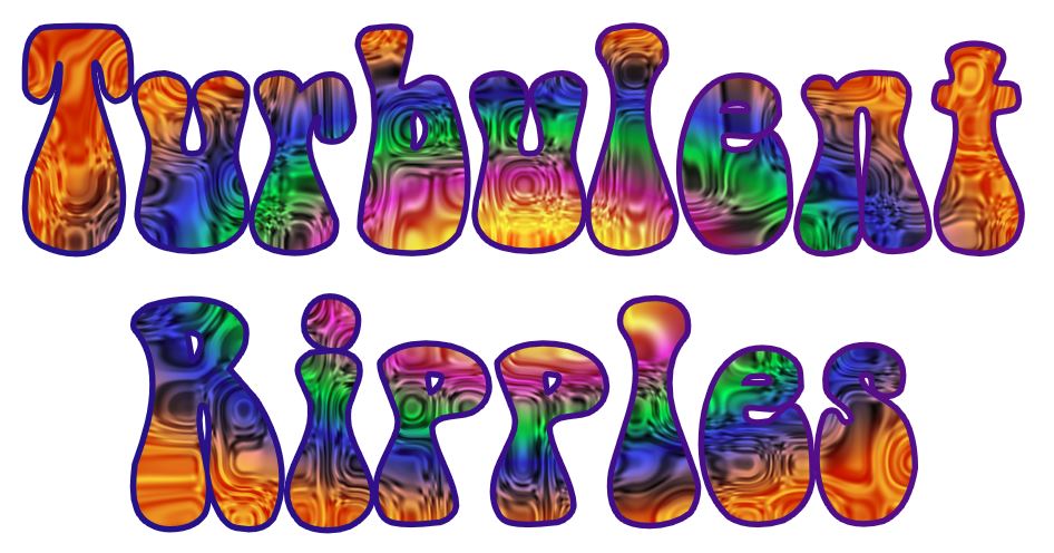
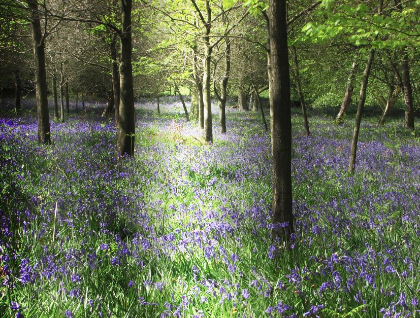
USING BRACKETS IN EQUATIONS PART 1. The previous lesson is HERE Introduction In the last lesson we looked at how to substitute controls (Custom Inputs) for numerical values in equations, giving you the ability radically change the appearance of textures. The example equation we looked at was Affinity’s Simple Perlin Noise preset whose equation looks like this: perlinsc(rx/200,ry/200,7,0.6)*0.7 We saw how the *0.7 at the end of the equation affected the brightness of the texture and substituted the 0.7 with a slider custom input. This gives the ability to slide the brightness from the default maximum level of brightness down to black, but what if we want to go the other way? What if we want to take the default brightness of a texture and go brighter? In this lesson we’ll look at how simply adding a pair of brackets will give you better brightness controls of your procedural textures. Using this technique on the Perlinsc Noise Maker will give you custom grunge texture maker capable of producing textures like these: We will also see how to add brackets in the middle of equations, which can alter the way the texture appears. Don’t Be Sacred of Brackets! Above, I said that brackets – () – will improve brightness controls in your Procedural Textures, this is because in the equations, brackets are used to change how Affinity interprets what to do with the equation. Let’s go back to a bit of maths we all learned at school with this sum: 2x3+2 (or 2*3+2 in Procedural Textures, since they use * for the multiplication sign) The answer here is 8 because it is worked out like this: 2*3=6 then 6+2=8 BUT add a pair brackets to the sum and you get a different result: 2x(3+2) Now the answer is 10. Why? Because anything in brackets is treated separately. So now the sum goes like this: 2 times whatever is inside the brackets. What’s inside the brackets? 3+2 which equals 5. 2x5 equals 10. This basic principle of putting stuff inside brackets to change the way an equation works is the same with brackets in Procedural Texture equations. When Affinity sees stuff inside brackets it goes, “Hey, wait minute, I’ll do the stuff inside the brackets separately, and then I’ll do the other stuff.” You don’t particularly need to understand the maths or how brackets work in C++ coding (unless your into either), you just need to be aware that using brackets can radically change a texture, helping you find new and interesting textures for your projects – as you’ll see! Why is this important? Take a look at this equation I tweaked from one of Affinity’s default presets: perlincubic((rx+500)/((w*2)/b),(ry+500)/((h*2)/c),7,a It looks really complicated with A LOT of brackets, but it started off as good old Simple Perlin Noise (perlinsc(rx/200,ry/200,7,0.6)*0.7) We’re going to look more closely at this equation in the next tutorial. The point is that once you get your head around brackets you can look out for them in existing equations to see if there are any obvious ways to change what’s inside; whether you can change or substitute anything like numbers for Custom Input controllers. Equally, you can add brackets to equations to change how the texture works. This is where we look more closely at the *0.7 part at the end of the perlinsc(rx/200,ry/200,7,0.6)*0.7 equation which we’ve already discovered sets the brightness level for perlinsc noise. Note: Whilst this seems to be the case for noise functions, in other functions, e.g. the “sin” function, it controls other features. A Better Brightness Control Create a new canvas 1920 x 1080 pixels (although, like vector graphics, the dimensions and resolution don’t matter with Procedural Textures since they are generated by the equation). Create a new layer via Layer>New Layer (or click the chequerboard icon at the bottom of the layer palette) Fill with your foreground colour via Edit>Fill with Primary Colour. Add a Procedural Texture filter either as a live filter or through Filters>Colours>Procedural Texture and select the Perlinsc Noise Maker preset you made in the last lesson. If you don’t have that saved, you’ll need to go back to the previous lesson and create it now. It should look like this: As you can see, the last Custom Input control we added in the bottom section was a 0,1 Custom Input with the value e which we called Brightness. The equation reads perlinsc(rx/a,ry/b,c,d)*e. Sliding the brightness control fully to the right, it maxes out with a few pure white patches like this: TIP: Custom Input values don’t have to be single letters. Delete the e at the end of the equation and substitute it for br (for Brightness), and then change the e at the beginning of the Brightness custom input slider also to br. You could just as easily call it spiderbum, if you were so inclined – just so long as the value name in the equation matches the value name in the custom input. Stick with br for the moment. By putting the br in brackets we can multiply, divide, add or subtract the default level of brightness by any number we choose, making the texture brighter or darker. In practice, I’ve found * (multiply) and / (divide) to be the most useful for adding more control to brightness levels. To begin with, lets double the brightness. To do this, we simply times br by two, but enclose in brackets so the equation now reads: perlinsc(rx/a,ry/b,c,d)*(br*2) The texture should be a lot brighter. Because it is DOUBLE the brightness, sliding the slider back half-way returns the texture to its default level, whilst moving the slider to the right of centre makes the texture lighter than the default setting. If we use / (divide) instead of * (multiply) we get the opposite effect. / (divide) makes the texture much darker to start with. perlinsc(rx/a,ry/b,c,d)*(br/2) with the slider fully right means that the starting brightness value is now HALF its default value. Make Some Grunge Let’s go really bright. Instead of multiplying br by 2, multiply it by 20 so that the equation now reads: perlinsc(rx/a,ry/b,c,d)*(br*20) (multiplying the default brightness level 20x) Change the Custom Input values as follows: Width = 15 Height = 15 Softness = 7 Detail = Set the slider midway Brightness = Set the slider midway You should have something that looks like this: Save this as a Preset. Click on the burger icon at the right-hand end of the Equation Preset drop-down list. Call this preset Perlinsc Grunge Maker. You could save it one of the categories we made in previous lessons or create a new category just for grunge. NOTE: You get some really wacky results if you multiply (*) or divide (/) the brightness by huge numbers like 1,000,000. Before we move on to another example, make a note of these grunge variations: Grunge Variations Try these different variations. Each one can be saved as a sub-preset by clicking on the burger icon at the right-hand end of the Custom Inputs Preset drop-down list. Sand Width = 2 Height = 2 Softness = 5 Detail = Set the slider to about 90% Brightness = Set the slider to about 1% Test this texture out by adding a new Fill Layer above the texture layer with an orange-yellow as the fill colour, then flip through the various layer blend modes to see the effects. Large Grubby Marks Width = 500 Height = 500 Softness = 9 Detail = Set the slider to about 100% Brightness = Set the slider to about 100% Remember that the rx and the ry in perlinsc(rx/a,ry/b,c,d)*(br*20) means that you can click on the texture and drag it around to find other areas of the texture. Two different areas of the Large Grubby Marks sub-preset. Weathered Wood Grain Width = 5 Height = 600 Softness = 25 Detail = Set the slider to about 90% Brightness = Set the slider to about 1% Another Example of Using Brackets Undo everything you’ve done so far, going back to the new document with a filled pixel layer, then add the Procedural Texture filter. If you’ve got the Procedural Texture as a Live Filter layer, double-click on the icon for the Procedural Texture (a black hourglass on a white background) to reopen the Procedural Texture Dialogue. From the Equations Presets dropdown list, select Ripples in the Monochrome Patterns category. The equation looks like this: var v=vec2(rx,ry)*(c/w); noisesc(v+(udirsc(v)*t)) This texture has two Custom Inputs (c and t) called Square Count and Turbulence. There are already quite a few sets of brackets is this equation: (rx,ry) we know make it click-dragable. (c/w) divides whatever number is in the c input (50) by w – which C++ code for width. All this front section - var v=vec2(rx,ry)*(c/w) - is doing is setting a value for the letter v in the next section. The next section takes whatever value for v is to help in the making of noisesc noise. The second section of the equation - noisesc(v+(udirsc(v)*t) – is where the action takes place. It is making noisesc noise, guided by the v value and using the udirsc function to stir the pattern up (make it turbulent). The amount of turbulence is controlled by the t Custom Input. Mix Things Up The turbulence controller, t, is a good place to start. We can make the texture really gnarly if we multiply that t by a number like 25. t*10 multiplies the turbulence set by the t Custom Input by 10, BUT WE HAVE TO ENCLOSE IT IN BRACKETS. Edit the last part of the equation so it reads: var v=vec2(rx,ry)*(c/w); noisesc(v+(udirsc(v)*(t*10))) Note the number of closing brackets at the end. That’s a MUCH more interesting texture! If you wished, you could save this as a preset called “Turbulent Ripples” in the Monochrome Patterns category. In the image below, I set the Square Count to 20, applied it to some text, added an elliptical layer fx gradient set to hard light and added an Outline, also via layer fx. Go Large Looking at the equation, thus far we have: var v=vec2(rx,ry)*(c/w); noisesc(v+(udirsc(v)*(t*10))). The segment of the equation (c/w) takes the width w and divides it by whatever number is in the Custom Input c. What happens if we want to see what happens when multiply w by a number like 200? The sum, or expression, to do that is straightforward – w*200 (width time 200) – but you can just slap that in after c/w like this: c/w*200. Affinity will take c, divide that by width w and then multiply the result by 200. Instead, we put brackets around w*200 to let Affinity know we want it to treat that bit separately like this: var v=vec2(rx,ry)*(c/(w*22)); noisesc(v+(udirsc(v)*(t*10))). The difference the brackets make could not be more dramatic: WITHOUT BRACKETS var v=vec2(rx,ry)*(c/w*200); noisesc(v+(udirsc(v)*(t*10))) PRODUCES THIS: WITH BRACKETS var v=vec2(rx,ry)*(c/(w*22)) PRODUCES THIS: Go ahead and add the expression in brackets so that the equation now reads: var v=vec2(rx,ry)*(c/(w*22)) You have now produced a click-draggable, scaleable AND distortionable lighting gradient. You can save this a preset as BW Adjustable Lighting Gradient. I have created a category for Lighting FX in which I save textures of this kind. Using the Lighting Gradient Open an image or download my Bluebell Woods from the files at the end of this tutorial. Go to Layer>Live Filter Layer>Colours>Procedural Texture. Select the BW Adjustable Lighting Gradient you just made. Click on the left side of the gradient and drag it to the right (towards the dialogue box). I was looking for something that might make an interesting effect and found this: It doesn’t matter if you can’t find the same section of the texture, just something with a bit of high contrast will do. At the bottom right of the Live Procedural Texture dialogue is the drop-down list for change the filter’s blend mode. Change it to Overlay. A dramatic shaft of light (or something similar). Play with the Turbulence and Square Count controls whilst dragging the texture around. Returning the Blend Mode to Normal can be helpful in finding other useful areas of the texture. With the Turbulence set to about 75%, and dragging around, I found this: Giving this effect of deep-shaded forest floor when the Blend Mode is changed to Colour Burn and the Opacity (bottom left corner of the dialogue) set to 50%: BRACKETS PART 2. IS HERE

DOH! Thanks for spotting that one. I have also just noticed that I have R controllers in the image not Z controllers - think I must have been asleep that day 😅.