Search the Community
Showing results for tags 'equations'.
-
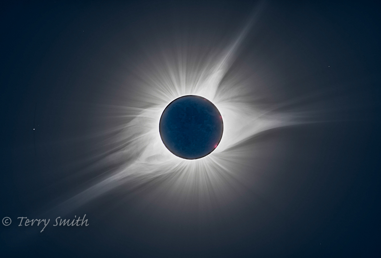
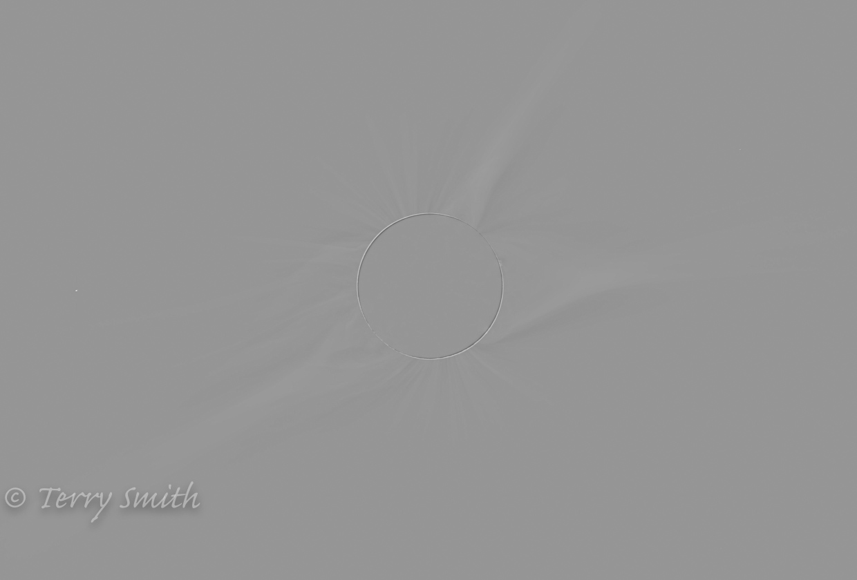
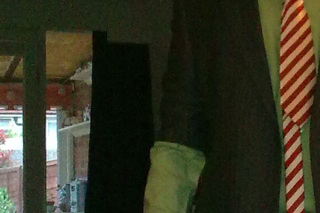
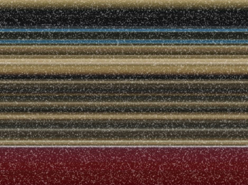
 First post here. I've been working on a composite of images captured during totality & getting some banding artifacts in PS when forced to use 16 bit mode rather than 32 bit for sharpening steps. I'd like to make sure Affinity Photos has the adjustments I need in 32 bit mode. The complete workflow for PS is describe in this tutorial by Russell Brown: PS Spin Blur Eclipse Processing From Photos tutorials, I see there are spin-blur filters, Apply Image: Equations panel & an Equations panel. So maybe everything I node is there but done differently in Photos. The key step I'm unsure about is in one of the equations panels. In PS, a duplicate image is spin blurred & the alpha channel of that image is subtracted from the original alpha w/ an off-set of 128 in the Calculations panel to give a low contrast mid-gray frequency mask. That mask is then Overlayed onto the original. I'd like to confirm that all this can be done in Photos in 32 bit mode? Here is a version of my PS work from 77 images w/ artifacts & a mask. The frequency mask reveals the finer corona detail. Thanks!
-
 This is an extension of my tutorial on Trigonometrical transformations using Filter > Distort > Equations. This one is focused on simulating flags waving in a light wind. Flags have an advantage in that they have a standard shape (width is twice the height). Edit: I have been told that this is not true. I stand corrected. To get the desired waving, I apply a sine transformation to each of the x and y-axes. The equations to apply are: x=(x+20*sin(360*y/h))/c-100*b y=y+a*(h/10)*sin(2*360*x/w)-(x/w)*h/10 I add a sideways sine wave to the x-axis as a function of the y-position. When the flag waves, the visual width is decreased, so I have added a parameter c which scales the width of the flag. The parameter b is an offset, since the left-hand corners of the flag can otherwise move outside the canvas. The y-axis also has a sine wave, depending on the x-position. The parameter a determines the magnitude of this sine wave. The final expression (-(x/w)*h/10) ensures that the fly (RHS in this case) is below the hoist (LHS here). (Definitions: hoist is the part next to the flagpole; fly is the part flying free.) Here is the UK Union Flag, plus a bit of extra space above and below to create room: And waving in the breeze: And here is a macro that implements these transformations: FlagWaving.afmacro And a macro library containing the single macro: FlagWaving.afmacros The parameters should appear when you run the macro. Parameter a controls the vertical wave; parameter b controls the horizontal offset; parameter c controls the overall horizontal scaling. This macro will not simulate a flag in too strong a wind, where the parts overlap! John
-
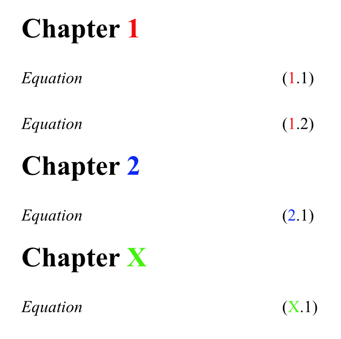
 Hello, I have a big request. I have run into a problem with the automatic numbering of equations in Affinity Pubhlisher. I would need to create an automatic numbering for math equations so that the first number corresponds to the chapter number in which the equation is located. I am attaching an image for visualization. Thank you in advance for all the advice! Viktor
-
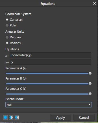
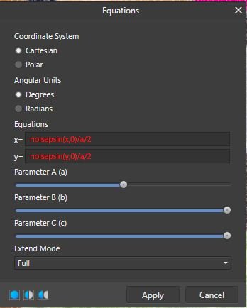
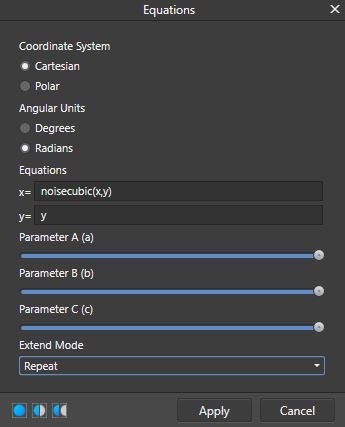
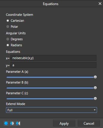
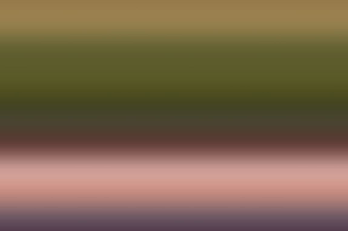
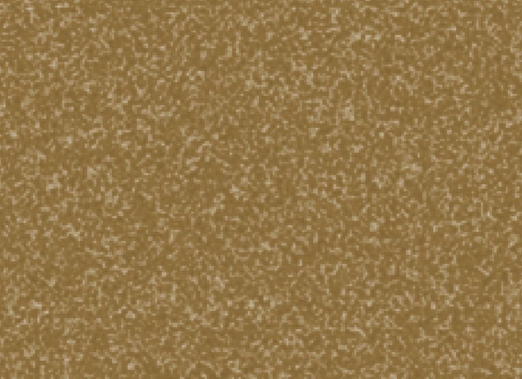
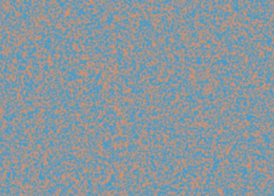
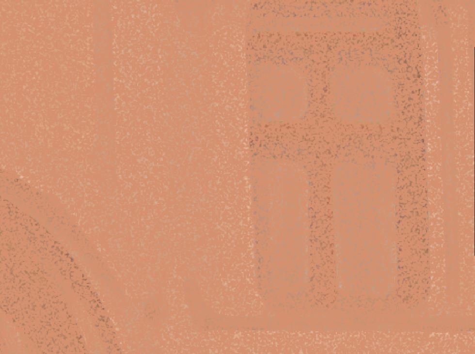
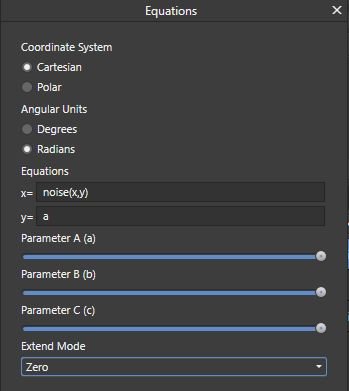
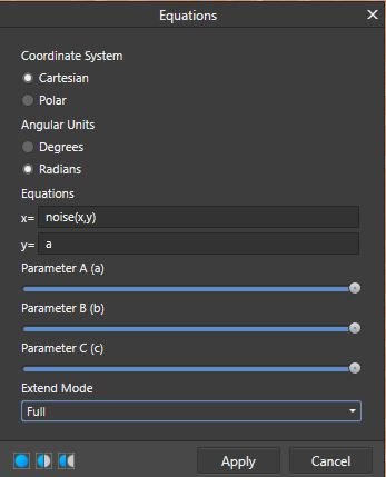
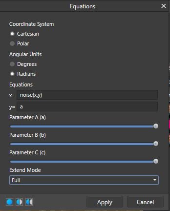
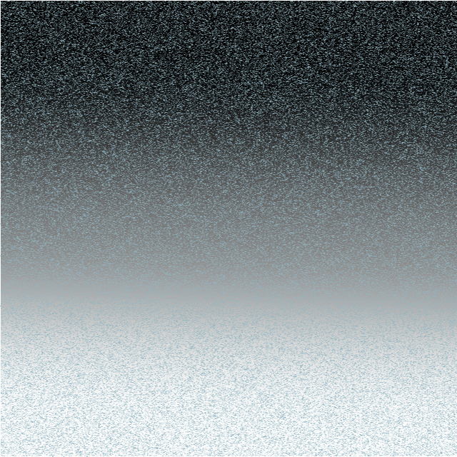
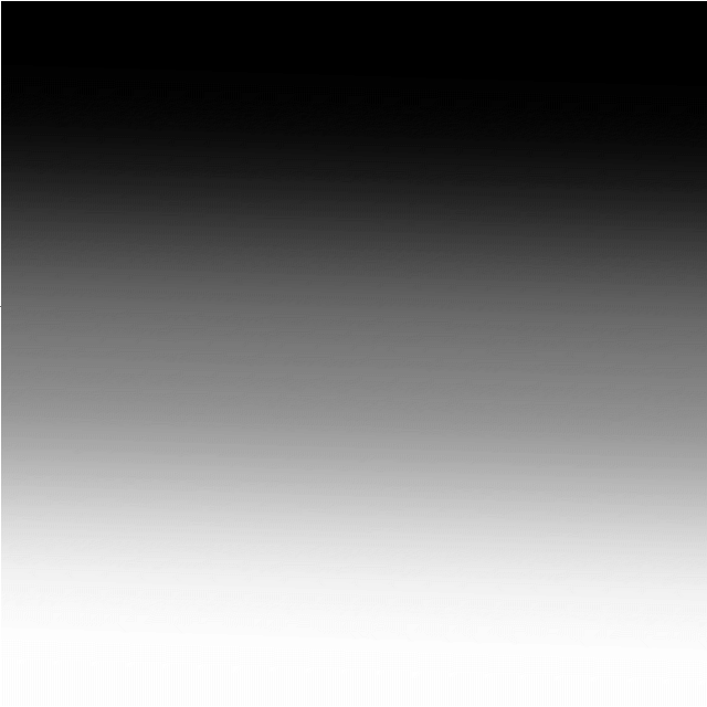
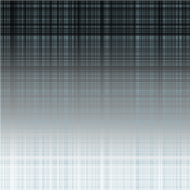
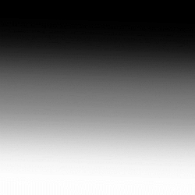
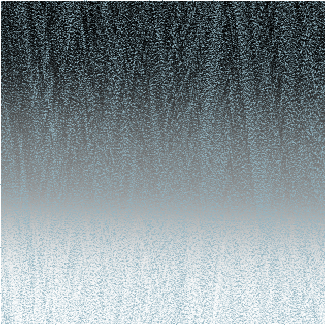
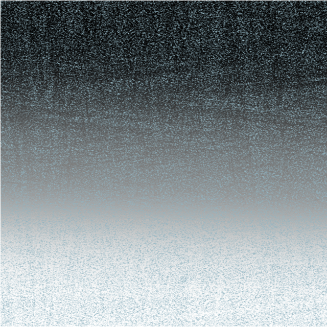
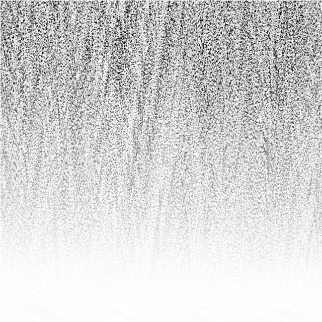
 Part 1 of this tutorial which explains what procedural noise is and how it works can be read here. Introduction What follows are a few examples of how noise can be used practically and creatively. We will set up a couple macros to save for future use. If you aren’t familiar with macros, you can still follow the steps ignoring the macro parts. Alternatively, you can learn how to use macros on Affinity’s YouTube channel here. Before we launch into creating the macros, one, key discovery I’ve made which makes noise equations far more useful is that Equations noise can be generated on an empty pixel layer. Let’s do this now, so you can see what I’m talking about. Create a new, empty pixel layer above the background layer. Go to Filters Menu>Distort>Equations. Enter the basic noise Equation in the x= box – noise(x,y). Leave the default letter y in the y= box. Nothing happens! BUT… Change the Extend Mode to Full. Click Apply. Now you have a non-destructive noise layer of light “noise” type noise. If you want dark noise, just invert the layer. This layer can now be changed with layer blend modes (Overlay & Soft Light), rescaled, tinted, blurred, opacity reduced etc. Now we’ll create a couple of useful noise Macros. Add White Noise Macro Let’s use a different form of noise (noisecubic) to create a macro which will add white noise to images. First delete all layers apart from the background layer. Open the Macro tab and press the record button to start recording. Create a new pixel layer. Go to Filters Menu>Distort>Equations Apply the following equation: x= box - noisecubic(x,y) y= box - y Extend Mode - Full Click Apply. Change the noise layer’s name to White Noise. Press the stop button on the Macro tab. Save the macro as “Add White Cubic Noise” (without the quotes). Note: Hit the “Add White Cubic Noise” button a few times to see the effect increase or try changing the “White Noise” layer mode to Overlay or Soft Light. The effect of using the Add White Noise macro 3x Add Dark Cubic Noise Macro Follow all the steps for Add White Noise above but invert the White Noise Layer layer at the end and change the name of the noise layer to Dark Noise then save the macro. Controllable Weave Textures Early on in this tutorial we saw how putting the equation noise(x,1) in the x= box and a in the y= box generated vertical bars of averaged colour when applied directly to a photo pixel layer. If, instead, we apply the same equation to an empty pixel layer above a filled pixel layer, we have the foundation for creating a Weave texture (many textures, since there are so many types of noise). To create the macro, do the following: First delete all layers apart from the background layer. Open the Macro tab and press the record button to start recording. Create a new pixel layer. Go to Filters Menu>Distort>Equations Apply the following equation: x= box - noisepsin(x,0)/a/2 (note: 0 is the number zero, not the letter O) y= box - noisepsin(y,0)/a/2 Set the Parameter A to the midpoint. Set the Extend Mode to Full. Click Apply. Change the name of the layer to White Weave Texture. Save the macro as White Weave Texture. The Weave Texture – which shouldn’t work, since it’s all red – but it does! The weave texture equation explained: “noisepsin” is just the command to generate noisepsin type noise. (x,0) in the x= box tells Affinity to only make noise in the x direction (left to right, I think) (y,0) in the y= box tells Affinity to only make noise in the y direction (top to bottom, I think In both boxes the 0 (number zero), I suspect, is the amount of offset from the starting point in the top left-hand corner. Certainly all changing this number does is change the pattern ever so slightly. /a – The / sign means “divide by”; the letter a activated the Parameter A slider. /2 means “divide by 2”. Purely by experiment I found that multiplying the equation by a (noisepsin(x,0)*a) made the Parameter A slider have the effect of gradually filling the transparent areas of the texture with white when the slider was moved to the left. Dividing by 2 (noisepsin(x,0)/a), on the hand, had the effect of make the Parameter A slider gradually reduce the number of stripes as the slider was moved to the left. Dividing everything by 2 (/2) at the end meant that the default position of the equation is now half-way along the Parameter A slider. Moving the Parameter A slider left gradually decreases the amount weave; moving it right increases the amount of weave. So, the whole equation instructs Affinity to generate noisepsin noise, from left to right, and from top to bottom separately (creating vertical and horizontal stripes), but the amount of noise is going to be controlled by the Parameter A slider. Weave Texture applied to the test image – the layer mode was set to Overlay. Adjustable Gradient Background from any Image This macro will generate adjustable gradients from any image. To create the macro, do the following: First delete all layers apart from the background layer. Open the Macro tab and press the record button to start recording. Duplicate the layer with Ctrl+J. Go to Filters Menu>Distort>Equations Apply the following equation: x= box - noisecubic(x,y) y= box – y Extend Mode – Repeat Click Apply. Go to Layer menu>New Live Filter Layer>Blur>Gaussian Blur IMPORTANT: Make sure you put a tick in the Preserve Alpha box, or the blur will not go to the edge. Set the Radius to 50px. Close the Live Gaussian Blur Dialogue (Don’t Merge, Delete or Reset). Select the Gaussian Blur’s parent layer (should be the top layer). Rename this layer as Gradient Blur. Press stop on the Macro recording tab. Save the Macro as Horizontal Gradient from Image. When you run the macro on any photo or image (must be a pixel layer, don’t forget), it will generate a horizontal gradient with a live blur which you can adjust. Gradient produced from the test image with Gaussian Blur set to 100px See if you can create a macro which will generate a vertical gradient. Adjustable Coloured Noise This macro creates a layer of coloured where you can choose any colour at any brightness or saturation level. It uses the same steps as the horizontal gradient macro, but with a few tweaks. To create the macro, do the following: First delete all layers apart from the background layer. Open the Macro tab and press the record button to start recording. Duplicate the layer with Ctrl+J. Go to Filters Menu>Distort>Equations Apply the following equation: x= box - noisecubic(x,y) y= box – a Extend Mode – Full Click Apply. Add a new HSL Adjustment Layer. Close the HSL Adjustment Layer Dialogue (Don’t Merge, Delete or Reset). Select the layer beneath the Adjustment Layer (choosing “Select 1 layer below current”) Rename this layer as Coloured Noise. Save the Macro as Coloured Noise. To use the macro, run it, then drag the HSL adjustment layer onto the Coloured Noise layer. You will then be able to adjust the coloured noise without affecting layers underneath (double-click on the HSL layer icon). Conclusion I hope I’ve show that using noise in the Equations filter is: a.) less scary than you thought, and b.) genuinely useful, with many potential applications. Note to Affinity developers – It would be sooooo helpful if the next release of Affinity had the ability to save Equations as presets in the same way as the Procedural Textures filter. That would save having to use macros and make them even more practicable.
-
- 3
-

-
- equations
- how to use
- (and 8 more)
-
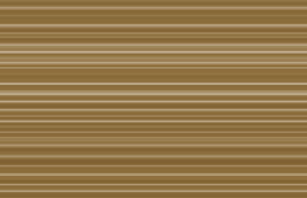
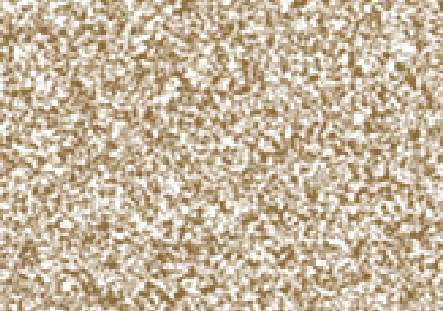
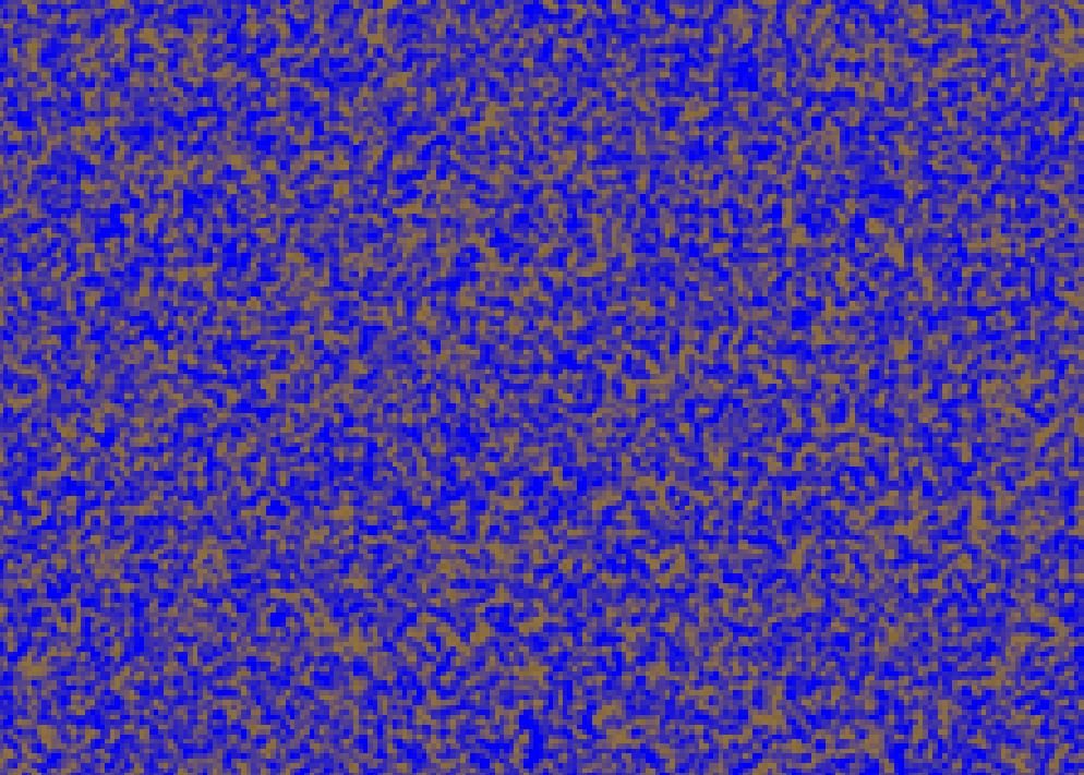
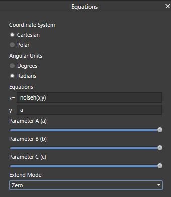
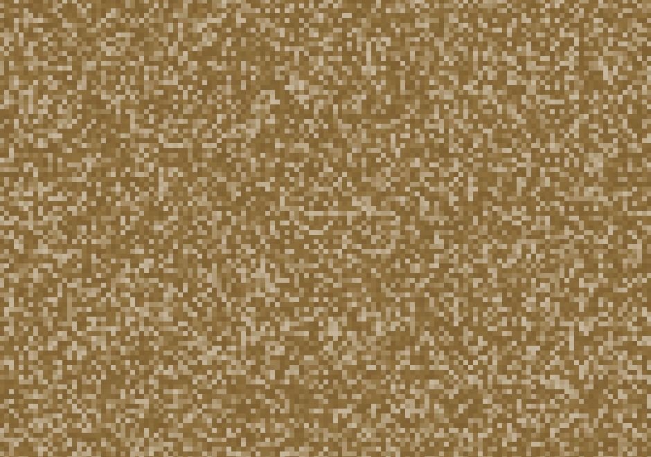
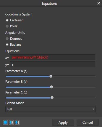
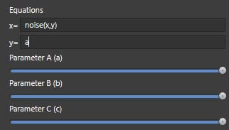
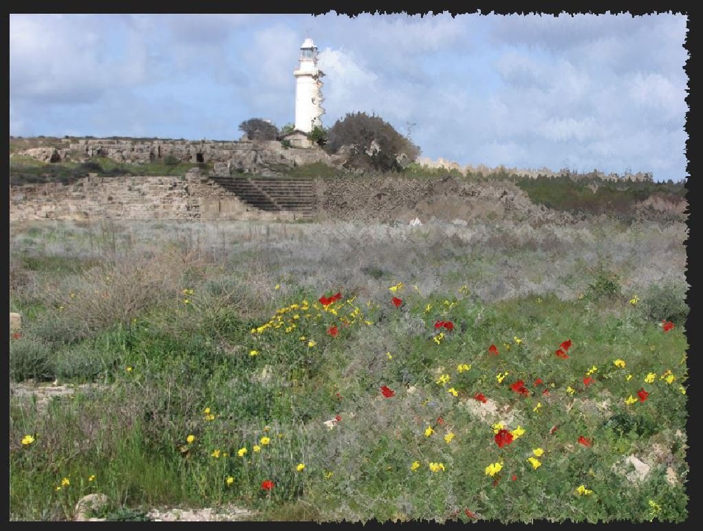
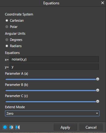
Summary This tutorial: Is aimed users with little or no knowledge of the Equations filter. Explores what “noise” is, in the Affinity Photo filters – particularly how it appears in the Equation filter. What the effects of “Extend Modes” have on noise generated in the Equations filter. What the effects are of using the “a”, “y” or other equations in “y=” part of the Equations. Shows how noise equations can be used effectively on an empty pixel layer. Offers some practical uses for noise equations with macros. Introduction The aim of this tutorial is to explore the inner workings of the “noise” command as it’s used in the Equations filter in a practical and experimental way. I am not a computer programmer or a mathematician – so this is layman’s perspective, not a technical tutorial. The goal is to help users who have only a rudimentary understanding of the Equations filter get to grips with and find uses for the noise function in the Equations filter. Hopefully, any inaccuracies will be picked up by other users in comments. I’d like to thank John Rostron, whose more technical article about the noise function made me curious – you can read it on the forum HERE. Preparation If you want to follow in Affinity Photo the experiments I’ll make in this article, you’ll need to do the following: Open a test image or download mine – link at the bottom of the article. Make sure the image is a pixel layer not an image layer. If it says “Image” on the layer in the layer palette, right-click and select “rasterise…”. Duplicate this layer with Ctrl+J. Create a new pixel layer above the bottom Background layer and fill with a blue colour (eg. R:0, G:0,B250). This will enable you to see any transparent areas made by noise in the top layer. Noise vs Procedural Noise So, what is “Procedural Noise”? In digital imagery like digital photos and scanned images, noise is unwanted artifacts in the form of random variations in the colour and tone of pixels in an image, which are not part of the original image. They are generally produced as a result of electronic interference. If you push the ISO on your digital camera to its highest rating and take a photo in low light, zoom in and you will likely see spots, speckles and coloured patches which were not a part of the scene (see image below). A noisy image produced on a high ISO on an older camera. Usually (and mainly in photography) this noise is unwanted, but it can be used creatively for special effects or for artistic purposes by graphic designers and artists, so software like Affinity Photo usually provides effects filters which let the user add various forms of noise to their images. This noise is produced by a mathematical algorithm or piece of computer code, and so is made by a procedure – hence “Procedural Noise”. Here are couple of examples of procedural noise used artistically: In the image above, I used the Filters>Noise>Perlin Noise filter in combination with the Displace Filter for a quick artistic effect on the right-hand side – the left side is the original image. Both the background and the text textures in the image below were created using noise equations in the Equations filter. Affinity Photo provides the user with four main ways to introduce noise, all found in the Filters menu. Add Noise… and Perlin Noise… are found in the Noise section of the Filters menu. These are the simplest way to add noise, since they have a user-friendly interface. Noise can also be introduced through the Procedural Texture and Equations filters found in the Colours and Distort sub-menus. Both these require the user to enter equations, which can make them seem daunting, if not a no-go area, as there virtually no guidance on how to use them in the help file for those without any technical knowledge. If you want to begin understanding and using Procedural Textures in an accessible way, try my absolute beginner’s tutorials here – which also uses noise functions. Procedural Textures – Key Features The single most important/useful thing about procedurally produced noise is that it can be produced at any scale or resolution of image without degradation. Because it is a random pattern (pseudo-random, if we’re being pedantic) produced by an equation, the pixels it produces are not fixed or ‘real’ until the apply button is clicked. Instead, like vector graphics, the work at all sizes and scales of image. You can fill a 1mp or 100mp image with noise and the pattern will never repeat or degrade. One feature I have discovered, which is often overlooked, is that procedural noise is composed essentially of two areas: areas with the noise pattern and the areas between, which I am calling negative space. It turns out, the negative areas are just as important as the bits of noise, as we’ll see later. More precisely, it seems that there are parts (pixels, ultimately) which are solid colour, and others which are increasingly transparent – which become more evident when using noise in the Equations filter. Let’s take a look at very basic noise in the Equations Filter: Check to make sure the top layer of the test image is still selected. Open the Equations filter dialogue by going to Filters>Distort>Equations. Enter the following equation exactly as it is in the with no capitals or spaces: In the x= box type noise(x,y) In the y=box type the letter a (Which I’ll explain later). From the Extend Mode list, select Full. Coordinate System should be Cartesian, and Angular Units should be Degrees, by default – from now on everywhere I describe inputting an equation in the Equations dialogue the default settings of Cartesian and Degrees will be assumed. DON’T click apply, leave the dialogue open so you can follow the experiments below. To see the noise more clearly, hold down Ctrl and scroll your mouse wheel forward to zoom in. You can now see clumpy, fuzzy blobs of solid colour with fuzzy white patches of negative space. Zoomed out, it’s the coloured bits that we perceive as noise. I’ll explain the reason for the strange colour in a moment. What’s going on? What’s really happening is that the noise command generates random vertical and horizontal bars of tone shaded from white to a solid colour. We can see this by changing the equation. At the moment noise(x,y) is an instruction to make noise in the x and y directions - horizontally and vertically. Change the equation so that it reads noise(x,1). You should see random vertical bars in various tones of colour like this. Now change the x in the equation to a y, so the equation reads noise(y,1). You should see random horizontal bars in various tones of colour like this. This indicates that noise(x,y) is really a blend of the two. What the deal with the colour? When the noise(x,y) equation is used in combination with the Full noise Extend Mode, the filter generate noise which is a kind of average colour of the whole image, though this is not exactly the same colour as would be produced by the Blur Average filter. From my experiments, these white areas are, in reality, appear to be areas of transparent and semi-transparent pixels, depending upon the tone of the pixels. Pixels of the true averaged colour are opaque whilst lighter tones are increasingly transparent, until you get to white which is entirely transparent. At the moment, we are seeing the light pixels as white because, in this instance, the Extend Mode we’re using is Full, which makes the white areas opaque. I’ll explain a bit more about transparency later, when we look at other Extend Modes. There’s more than one kind of noise! Until now, I’ve been using the word “noise” to talk about procedural noise in general terms. In fact, in the Equations Filter the word “noise” is the name of just one particular type of noise. In the programming language used to generate procedural noise in both Procedural Textures and Equations, there are dozens of different types of noise (noise, noisei, noiseh, noisecubic, noisesin etc.), each producing a slightly different type of noise. The differences are, perhaps, more noticeable in Procedural Textures where you can magnify them to create interesting patterns, effects. You can see the full list if you look up Procedural Texture in the help file. Scroll down the page and you’ll eventually come to the lists of different noise types. For a very different kind of noise add the letter “i” after the word noise, so the equation reads noisei(x,y) in the x= box (till with a in the y= box and the Full Extend Mode). This makes noisei type noise, which is blocky and pixelated. noisei type noise Now try substituting the letter “i” with an “h”, so you have noiseh(y,x) in the equations. You should end up with something like this: noiseh type noise You can now clearly see the coloured fuzzy blobs of noise with the negative white areas between. Extend Modes make a MASSIVE difference Let’s prove that white areas and lighter tones are, in fact, areas of transparency. Just to remind you, Extend Mode is last option at the bottom of the Equations filter dialogue. It contains a drop-down list with Zero, Full, Repeat, Wrap and Mirror. Each mode has a different effect upon what the equation does to the image. Change the Extend Mode to Zero. noiseh(y,x) with Zero Extend Mode. Suddenly, you can see the underlying image (the blue layer) through a veil of noise. Experimenting with different extend modes To experiment with different Extend Modes, we’ll use the first noise equation we started with. It should still be open, but if it isn't, set it up the Equations dialogue as follows: That letter a in the y= box essentially activates the Parameter A slider, turning it into a sliding controller. I’ll come back to this later. Try testing out the Equations with different Extend Modes, at the same time as sliding the Parameter A slider back and forth. Here’s what I observed. Zero Extend Mode produces noise with transparent negative areas revealing the layer underneath the current layer. The noise pixels are made more transparent by sliding the Parameter A slider to the left. There is an initial brightening of the noise before it begins to fade, never quite going completely transparent. Full Extend Mode fills the layer with white overlain with noise. The noise pixels are made more transparent by sliding the Parameter A slider to the left. Repeat Extend Mode produces sparse noise (with this image) on a solid field of averaged colour. Moving the Parameter A make the noise and background colour lighter. Note: in one image, I found that the Repeat Extend Mode filled the layer with averaged colour and zero noise. Wrap Extend Mode is unpredictable from images to image. In the image, it averaged colour noise on a background which is the inverse colour of the noise. Moving the Parameter A to the left changes the relationship of the positive and negative colours, intensifying the background colour whilst making the noise more transparent. Mirror Extend Mode, gives identical results to Repeat, in these experiments. Dealing with the “y=” box So far, we have only had the letter a in the y= box. That is because the the y= equation box cannot be left blank. It must contain a value of some kind; either a letter*, a number, or another equation (which I’ll come back to later). If you enter the letters a,b or c in the y boxes then the A,B or C parameter sliders become active, giving customisable control of Equation depending upon which extend mode you use. *note: only letters that have a function in the Equations filter produce a result when used alone in x= or y= boxes. I will list other useable letters at the end of the article. However, if you leave the default letter “y” in the y equation field, you get completely different results with different Extend Modes. Try the following tests using noisei(x,y) in the x= field and y in the y= field. You’ll need to zoom out at little to get an idea of what is happening (hold down Ctrl and scroll the mouse wheel backwards). You should see something like this. Zero extend mode (above) produces random horizontal bands of colours which are averages of the area the bands cover. The negative, transparent and semi-trasparent areas of the noise pattern punch holes through the current layer revealing the layer underneath. Full extend mode (above) produces random horizontal bands of colours which are averages of the area the bands cover. The negative, transparent and semi_transparent areas of the noise pattern are white instead of transparent. You need to zoom in to see this more clearly. Repeat and Mirror, both produce random horizontal bands of colours which are averages of the area the bands cover with little or no noise. The Wrap Extend mode (above) is a weird one. It creates the same horizontal bands of colour, but this time, the negative spaces are of varying colour, perhaps inverse complimentaries? Using noise equations in both x= and y= boxes Adding a noise equation to the y= box in addition to the one in the x= box has the effect of adding a second layer of noise to the image. The resulting noise is now similar to the earlier noise where we put an a in the y= box. If the y= box contains the same equation as the x= then the effect, though, appears to be to increase the contrast between noise and negative areas. However, if equation in the x= box is noise(x,y) and the y= box is noise(y,x), the effect is to increase the overall amount of negative/transparent/white areas. What this means is that you can overlay two different kinds of noise, if you wish. Try for example, using noiseh(x,y) in the x= box and noiseh(y,x) in the y= box. This concludes Part 1 of the tutorial. Part looks at putting all to use with some practical examples. Scroll down for the link to Part 2. Notes Useable letters which can be use in the x= and y= boxes a, b & c – activate the parameter sliders in the dialogue h produces light, near neutral noise - Try h+a and h*a in the y= box with various modes. x & y Noises with the letter “h” in their name like (noiseh, noisehpsin, noisehcubic etc.) create harmonic noise, which has greater negative areas. Special note re. Perlin Noise Perlin noise, which you may have come across in the list of noise types, is a particular type of noise invented by Ken Perlin, who was looking for a way to generate more natural/realistic looking 3D textures. It has a more “clumpy” look to it. When it is scaled in 2D imaging software like Affinity it can create wonderfully versatile natural-looking textures from clouds to hair and even wood grain. Sorry to say, I have yet worked out how to scale any noise in Equations. Nevertheless is still a useful variation of noise. The Perlin noise command requires four pieces of information to work properly. I don’t want to go into any kind of technical depth here, so just try the example below (note the position of the Parameter A, B, and C sliders): Explanation: Perlinsin – a type of Perlin noise. rx,ry – generates the noise. The r before x and y means you can click in the image and drag the noise around. a*10 – Activates the Parameter A slider which seems to control softness and brightness b – Activates the Parameter B slider, which seems to control softness and graininess. /c/2 _ Activates the Parameter B slider, which acts as a sort of contrast control, change the spread of midtone pixels. GO TO PART 2
-
 For the Equations option in the Distort filter, what are the functions/operators allowed? There seems to be no documentation on what is accepted. I see transcendentals but not much else besides +-*/^ basic math. I sure could use modulus and logs of some kind.
 -
 You can find Equations Filter in Filters > Distort > Equations Many thanks to @NotMyFault @John Rostron and @R C-R Leave your formulas here! x-noise(x) *500 | x-noise(y) *500 | x-noise(x,y) *500 y x-noise(x) * 500 * a y-noise(x,y) * 500 * b The value 500 is the offset distance. It can be replaced by w or h, then the offset distance will be equal to the size of the document in width and height. x-w*a y-h*b Also below is an example of the dependence of A from B x-noise(x)*w*a*b y-noise(y)*h*b
-
 I think it would be nice to be able to store distort equations in a similar way to the procedural texture equations preset panel. At the moment it seems the only way to store distort equations is to either jot them down in another app somehwere, or store them in a macro. When you store them in a macro you lose the equation, so you can't go back to it, which is kind of annoying. I've currently got my equations building up a text document, but working like that doesn't fit the nice workflow that the other features have. Also, with the procedural textures panel if you accidentally apply before storing the preset you lose the equation, would it be possible to have a persistent edit buffer that populates the dialogue with the last equation you used, rather than it opening with a blank panel each time? It's really easy to spent time messing about to get an interesting pattern and then pressing apply to see the pattern properly (with the anti-aliasing in place), before saving it as a preset ... then it's gone, you've lost all that effort!
- 7 replies
-
- 3
-
-
- procedural
- equations
- (and 2 more)
-
 Hello there, in the tutorials equations are mentioned a few times, like in the Macros videos. But there is no general overview of the functions that I am aware of - for instance, relative to noise the video mentions that there are 4 different noise generators but I didn't find specific explanations as to possibilities using equations. Is there anything? I'd be glad to go through it...
 -
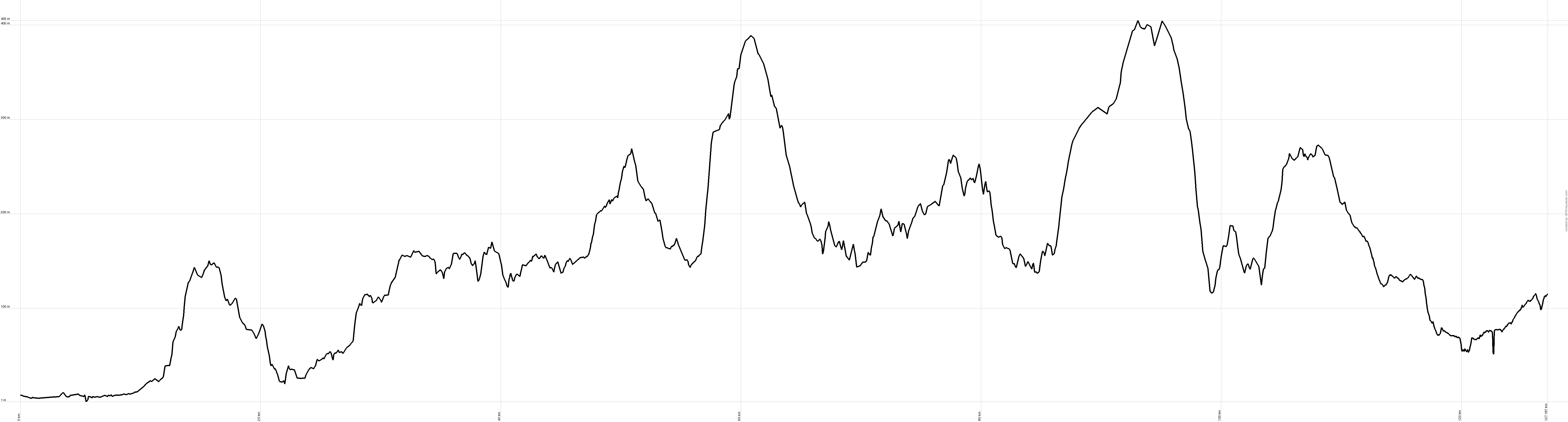
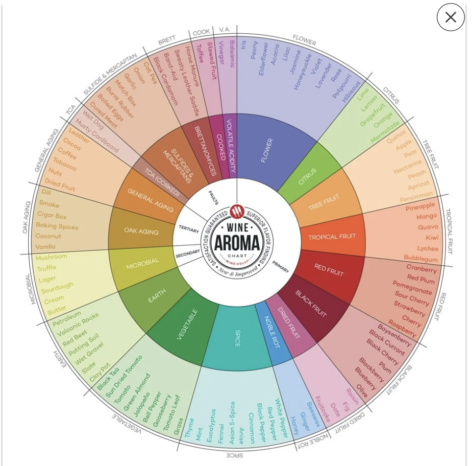
 Hi Affinity Community, I am looking to create a circular visual with text and a profile (which shows elevation and distance) that curves around the edge. I have been looking at this thread: https://forum.affinity.serif.com/index.php?/topic/131951-text-alignment-in-shapes/&tab=comments#comment-726530 And have found useful info for setting out and aligning text. I am also looking to warp this rectangular image onto the outside of the circle. I'd want to adjust the scale of it, so would transforming into a donut would be the best way to manipulate it? These would eventually go around the whole perimeter, I could either stick them together and warp one image, or ideally go around the segments adding another elevation profile. One elevation profile is attached (I have 12 of these) and an example of the final image I am aiming for. I'm using Affinity Photo. Thanks.
-
When using Filter > Distort > Shear, I can move the nodes by dragging or using the arrow keys. However, it would be good if I could enter formulae to describe how a node moves. For many purposes, this would be much more convenient than using Filter > Distort> Equations (which can do the trick). I have reported in the Bugs forum that moving the nodes with the arrow keys has a bug. Thanks to @MxHeppa who raised this problem in my thread on Warping Test onto a Wave. John
-
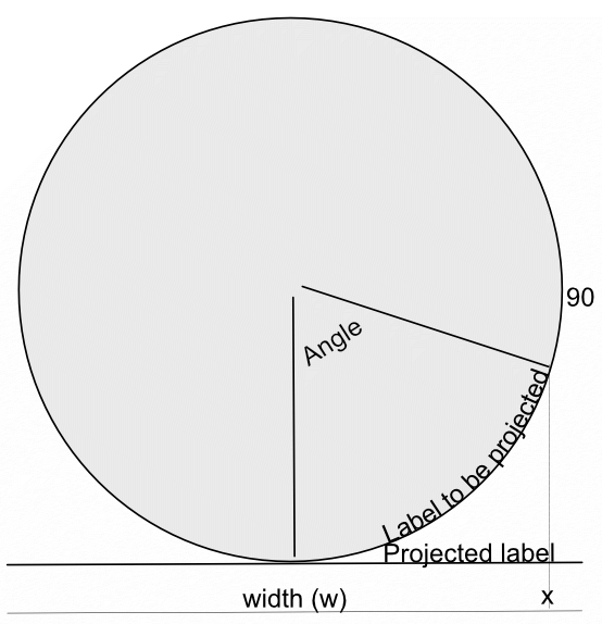
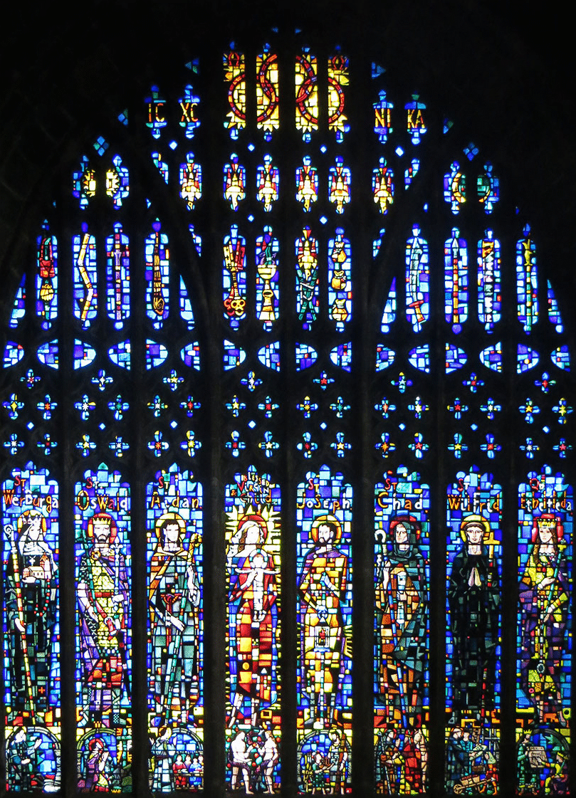
In a recent post in Questions, @Maxxxworld asked how he could warp an image to apparently wrap it around a bottle. I posted a solution to his problem there, which I expand upon here. Consider the facing semicircle of the bottle as seen in this diagram: The visible part of the label extends from -90 degrees (on the left, not shown) to 90 degrees on the right. This will correspond to the width of the original image. This will project onto the final width of the image (the line below). The final width is less than the original width by a factor of pi/2. A bit of trigonometry shows that the sine of the Angle indicated is given by (x-halfwidth)/halfwidth, where halfwidth is both the label and the final image. Putting this together and re-arranging a bit gives us an Equation: x=(asin(2*x/w-1)*w/180)*pi/2+w/2 A bottle is typically viewed from above, so that the label has a curve, typically with a dip in the middle.This can easily be simulated using equations, using: y=y-Const*x*(w-x)/w/w The Constant determines the depth and direction of the curve. I have used the expression w*(0.5-a) as a scaling factor, where a is a parameter chosen at runtime. This will change the curve from negative (curving down) at the default a=1 to positive at a=0. Inserting this into the equation gives: y=y+(0.5-a)*x*(w-x)/w Note that the w in the numerator and denominator cancel out. The value of (0.5-a) determines the curvature as described above. As an example, here is the Great West Window of Chester Cathedral. I chose this because it has lots of verticals to see how the filter affects it. (It has verticals once I had put it through the Mesh Warp.) And here is the image after the filter: Before filtering I cropped it close to the sides of the window and then Rasterized it to remove the invisible sides. I then added space at the top and bottom to allow room for the curvature part to operate. I then followed this by Clip Canvas to remove surplus transparent ends. The calculations for this filter are complicated by the algorithm that Affinity uses to effect these equations, which I explain in this Tutorial here. I have created a macro that effects the filter, and then uses Clip Canvas. By clicking on the cogwheel, you can alter the degree and direction of curvature. EDIT: I have discovered that this macro will only perform once (per Affinity Photo session). I add here a version recorded in version 1.8 which does work properly in Photo 1.8: WrapAround1.8.afmacro I alos onclude here the original macro, recorded in version 1.7: WrapAround.afmacro John
- 20 replies
-
- 14
-
-

-
 Hi, I am a scientist and Affinity Designer is my de-facto first choice for making illustrations for papers, posters, etc. Because it's great, and it's affordable. But making a scientific poster is a hassle. A true hassle. Because I do need to use equations. How does one import an equation into a Designer? I found several options, none really works for posters -- keep reading: 1) create a small LaTeX document; (a) compile into PDF; have hours of "fun" with fonts and import options. (b) alternatively, compile into a PostScript, open a file browser, rename PS into EPS, drag-and-drop, if you're lucky, sometimes I managed to make it work. Caveat: if you have many equations, they need to be in individual EPS files, otherwise Designer will not like one EPS file constantly getting changed. (Bonus: open your poster from a year ago with 20 EPS figures in it. Click 20 times on a popup window saying the source has changed because you re-ran the computer simulation which created them. After clicking on one popup, wait for a smooth animation as 19 other popups slide around your screen. Repeat 19 times. Then, you can access your poster. Probably.) 2) use online converters. The one I know that reliably works is www.codecogs.com . But it does not allow for fonts bigger than 20 pts, and fonts in posters are at least 24 pts. So when I really need to insert an equation I do this: (a) type it in codecogs, (b) download SVG file (copypasting from the browser results in a little black rectangle instead of the equation). So download the file, open the file browser, drag and drop. Not into the poster, that would be too easy. Because then, I'll need to manually resize the image to match my font size. I have devised some templates to insert the file into and either resize to match the size of a sample character, or type in numbers in Designer's "transform" tool, for which I need a calculator at hand (would be nice to download in 12pt and resize in Designer by 200%, but alas - so I use a calculator). None of this is a good working solution if you need like 20 equations. Is there a working solution? I have heard of LaTeXit, but that won't work in Windows. MS Office has some weird equation editor, but that won't copypaste to Designer. Every single time I make a poster, I often spend hours searching for other options online and it gets inexplicably frustrating. Every. Single. Time! When I need a lot of equations, I make a LaTeX save them all as a PS, then convert to EPS (they still have to fit on one page), then open it in a separate Designer window, then convert to curves, then "Group" curves corresponding to all symbols in a single equation, then resize in bulk, then copypaste. Aaarrrggghhh. Has anyone have found any working solution? As I said, the solutions above work if you have one equation, but are a true hassle if you need to put in a dozen. (Unless there is an alternative to codecogs that lets you set large font size and hopefully works as a copypaste?) It would be really great for more than just posters, as I often use Designer for illustrations, in which sometimes I need to use equations, too -- that would make me never want to quit the Designer ever. Thanks!
 -
 I managed to have an almost working solution to produce a pdf from latex containing text and equations that can be placed / opened in Affinity Publisher (and probably in Designer too, untested) as editable text. The example latex file `main.tex` needs to be compiled with lualatex (or xelatex, but pdflatex will not work), and requires the following OTF fonts: http://www.gust.org.pl/projects/e-foundry/latin-modern/download http://www.gust.org.pl/projects/e-foundry/lm-math/download/index_html I attach the produced file as `main_luatex.pdf`. Moreover, I opened the file with OSX Preview, and exported it as pdf with the name `main_exported.pdf`. Findings: - main_luatex.pdf + open / place in Affinity Publisher doesn't work (missing characters, ...) - main_exported.pdf + open / place in Affinity Publisher works as expected, text and equations are correctly imported as (editable) text - opening main_luatex.pdf in OSX Preview, copying and pasting text to Affinity Publisher works but the exact placement of equations is lost (expected); copying and pasting a selection (Tools -> Rectangular Selection) works but it ignores the selection box and the whole page is copied instead (unexpected) So, OSX Preview is doing something to the pdf but it's unclear what exactly. So I tried running pdffonts on the 2 pdfs but the only difference is in the number of objects: (base) ~/Downloads/tex $ pdffonts main_luatex.pdf name type encoding emb sub uni object ID ------------------------------------ ----------------- ---------------- --- --- --- --------- TIOITJ+LMRoman10-Regular CID Type 0C Identity-H yes yes yes 4 0 ZVNSJQ+LatinModernMath-Regular CID Type 0C Identity-H yes yes yes 5 0 ABULFO+LatinModernMath-Regular CID Type 0C Identity-H yes yes yes 6 0 (base) ~/Downloads/tex $ pdffonts main_exported.pdf name type encoding emb sub uni object ID ------------------------------------ ----------------- ---------------- --- --- --- --------- VZLAKC+LMRoman10-Regular CID Type 0C Identity-H yes yes yes 7 0 XSLNON+LatinModernMath-Regular CID Type 0C Identity-H yes yes yes 8 0 ZQHZQC+LatinModernMath-Regular CID Type 0C Identity-H yes yes yes 9 0 Moreover, while I can copy text from main_luatex.pdf and paste it correctly (equations aside of course) in an utf8-aware text editor, trying to do this with main_exported.pdf results in unrecognized characters (the dreaded square boxes). Which adds to the mystery as this is the file can be correctly imported in Affinity Publisher! Can someone with more expertise have a look at the 2 pdfs and explain what is the difference? I am aware that all these issues can (to some extent) be avoided by making any pdf "fontless" (i.e. using ghostscript to convert fonts to curves) but I need to work with text in my workflow for a number of reasons. In case there is a more relevant section in the forums please feel free to relocate this post as appropriate. main_exported.pdf main_luatex.pdf main.tex
 -
A useful addition to the Filter > Distort > Equations would be to have access to more than one layer. This would allow me to apply a function to the target layer based on what is in the second layer. It could be used for applying textures similar to displacement map. Obviously t would depend on the function being able to utilize the value of a pixel in the secondary layer. I see in a recent post that Affinity are working on a Macro Persona. I can'wait, but I won'hold my breath! John
-
In a discussion of creating a saturation mask, @dmstraker and @smadell referred to an equation involving channels: Saturation=(max(SR,SG,SB)-min(SR,SG,SB))/max(SR,SG,SB) The only way I can see to access these Source Channels is in Apply Image. However Apply Image deals with two images, a Source and a Destination. This calculation deals with just one. The information on Field Equations in Filter > Distort > Equations makes no mention of channels. How would I create a greyscale saturation layer from an RGB layer, which I can then convert to a mask? John
-
I wrote a macro to convert an image using a Cartesian to Polar conversion. It worked well in 1.6 and I describe it here. I have just tried it in the 1.7 beta and it no longer works. The output is a series of concentric colours, as if just the central axis has been rotated. I have tried running the original macro and also re-creating the macro with the same Equations. John
-
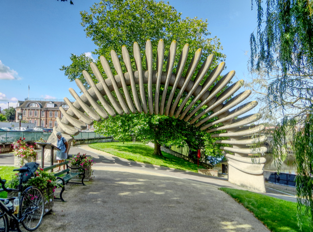
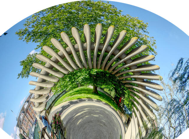
Conversion of a rectangular image to polar co-ordinates using Equations is not straightforward. A major problem is that the origin of the rectangular Cartesian co-ordinates is the top left, whereas for a polar display, you would typically want the origin on the midline, probably near the bottom. The following equations assume that the origin is in the midline along the x-axis, and at or near the bottom on the y-axis. First select Filter > Distort > Equations and enter: x=w*atan((x-w/2)/(h/a-y))/100+w/2 y=h-sqrt((x-w/2)^2+(h-y)^2) The expression (x-w/2) displaces the horizontal origin to the centre, and the expression (h-y) displaces the vertical origin to the bottom. In the first formula, for x, there is a parameter a, which allows you to scale the polar transformation; reducing the parameter a stretches the image around the circle. The 100 is an arbitrary scaling parameter which seems to work. The expression +w/2 at the end re-centres the image. This seems to be necessary, but I am not sure why. I would have expected to deduct w/2 rather than add it! Here is an original image of the Quantum Leap statue in Shrewsbury: With this transform using the default parameter a, this produces a quadrant. And with the parameter set to approximately 0.6: Here is the Macro: PolarQuadrant.afmacro The first thing the macro does is to unlock the image. I tend to do this automatically in macros. It is probably unnecessary. I ought to be able to give the adjustable parameter a, a name, but I have not been able to do this. John
-
WARNING: for the technically-minded only! The Noise functions in the Filters > Distort> Equations facility are supposed to add (unspecified) noise to an image. The only description I can find of this is in the video by James Ritson. He first duplcates the layer and then uses either noise(x*y)*a or noise4(x*y)*a in his equation. This produces a grain-like effect over his image. The documentation for equations is limited. There is the Expressions for field input in the Help system which gives, under : Noise(seed/x,y), an explanation: Generate 1D noise either from a seed or based on X/Y input with similar definitions for noise2, noise3 and noise4. James uses both the noise and the noise4 functions. In his video he is using the single seed parameter x*y, with the magnitude controlled by the a parameter. I have been experimenting with these noise functions and present here my findings Although the Expressions for field input names the functions Noise ... Noise4, with a capital letter, these will not work. You need to use a lower case n for noise. The function noise2 has no effect. The functions noise, noise3 and noise4 seem to produce identical visible results. The histograms are also identical. Using a single parameter, either a simple number, or an expression such as x*y, has no visible effect unless the Full option is selected in the Extend Mode at the bottom. When using two parameters, they need to be different in the x and y axes to produce any visible result. Multiplying the parameters by a number, such as noise(10x,10y), has no visible effect. I show here the effect of varying these parameters on a simple gradient field: Here is the effect of x=noise(x,y) and y=noise(y,x): The results for noise3 and noise4 are identical, as are noise(3x,3y) etc as are the histograms. If the parameters are the same, say x=noise(x,x) and y=noise(y,y) You get a very different effect: Almost like a tartan effect. If the noise functions are the same in both x and y such as x=noise(x,y) and y=noise(x,y), it works OK, but if you use x=noise(y,x) and y=noise(y,x) there is no visible effect unless you select Full: The difference between using Zero and Full in the Extend Mode at the bottom is subtle. Using Full seems to convert the image into a monochrome effect with the background invisible. However, the noise is based on the luminance of the background. Just for comparison, I append here the effect of the effect of the Add Noise filter (Filter > Noise > Add Noise...): You can control the intensity of the noise here, which is more than you can in any of the noise functions I have described. In conclusion, I would recommend that if you want noise, then use the Filter > Noise > Add Noise... option above until such time as the devs at Serif come up with a more understandable noise function in Equations. Having said that I am not holding my breath on this. Using noise in equations is probably a minority pursuit amongst users and the Add Noise filter is much easier. John
-
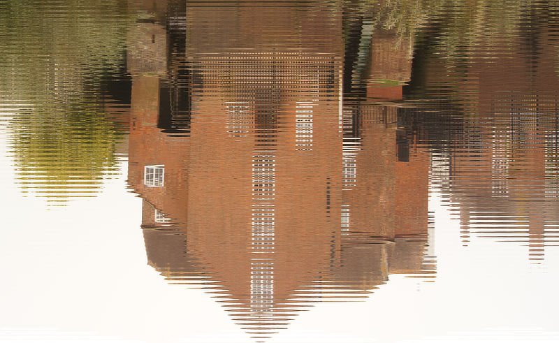
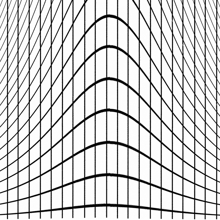
I was speculating on how Equations could be used to create a ripple-like effect in a reflection. I used an image of a Mill on the River Avon at Tewkesbury. I flipped the image vertically and then applied Filter > Distort > Equations as follows. The main effect is to vary the position of each pixel on the y-axis in a sinusoidal fashion, so I began with: y=y+100*sin(2*360*y/h) The 100 is just a scaling factor for now. This had the right effect but was the same right across the image, so I added a cosine function which would vary the magnitude across the x-axis: y=y+100*cos(10*x/w)*sin(2*360*y/h) Again the 10 here is a scaling factor. The result was: I should be able to tweak this into a macro where the user could vary the amplitude of the ripple, and the amplitude of the horizontal variation. A further tweak could be to add a perspective effect so that the ripples nearer the observer look larger than those further away. What do possible users think. Would this be a useful macro or are there easier ways to get the same effect? John
-
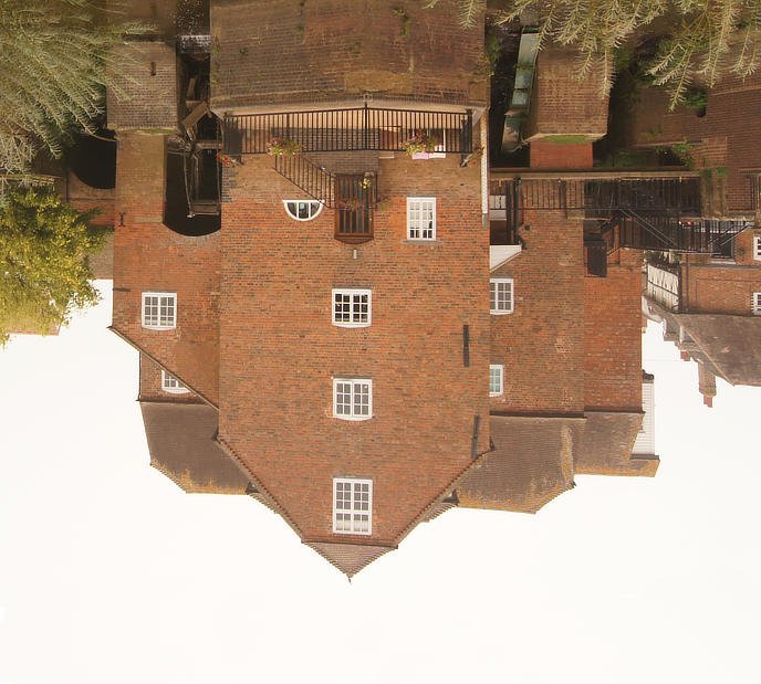
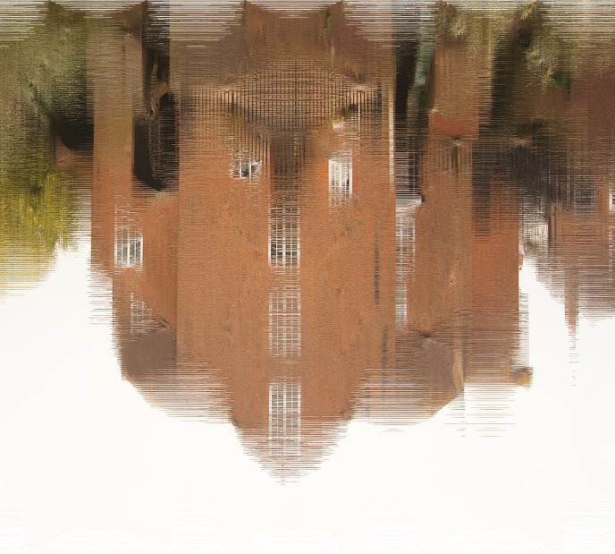
I have updated my Ripples macro originally posted under Tutorials. I am now posting under Resources, since it is really delivering a sort-of-finished product rather than a 'How to'. The new version has three parameters: a controls vertical spacing of the ripples. Reducing the a parameter increases the ripple frequency (reduces the wavelength). b controls the horizontal variation of ripple amplitude across the width of the image. Small values of b make the ripples change a lot across the image. For large values (~=1) the changes cycle two or three times across the image. c affects ripple complexity. This is very much a suck-it-and-see parameter. A value of one adds no complexity, a vale of 1 does. Here is an original image (Tewkesbury Mill inverted): And with the macro applid with a-1, b=0.5 and c-0.5: I have to admit that the results I have had with this macro are varied. Sometimes it is very impressive, but for other images it is definitely not! Here is the macro as a single file and as a library: Ripples.afmacro Ripples.afmacros I have been looking at the Distortions macro in the Macro Pack with mixed results. I have got it to perform, but not consistently. It appears to have no visible effect on the Tewkesbury Mill image. John
-
 I would ,like to be able to modify image RBG values based on combination of: a) neighbouring RBG values; b) user parameter inputs. I light to experiment with various colour abstractions of my images. I have not found any expressions in help material, or corresponding forum answers. Is this something already available? If so, where? Otherwsie could this capability be added to the equations/expressions capability of Affinity Photo.
 -
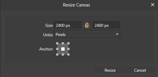
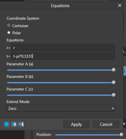
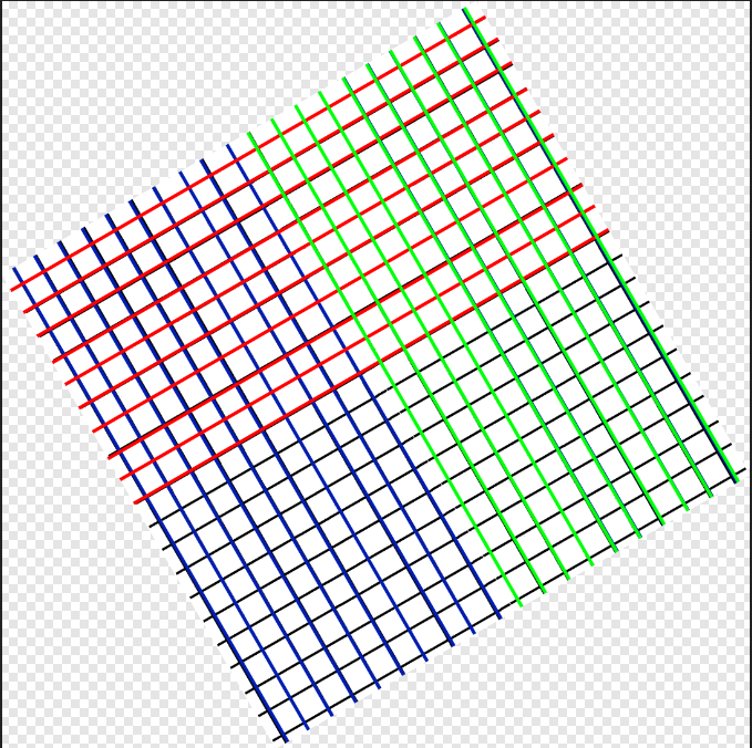
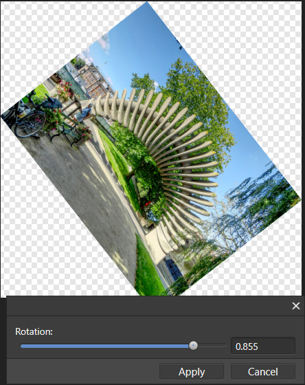
Many options for rotation in Affinity Photo are constrained to simple fractions of a circle, with 15 degrees being the smallest. It is possible to rotate by an arbitrary angle using the Crop tool. You place the cursor just outside a corner, and rotate by dragging the two-arrowed cursor that appears. This tutorial explains how you can rotate an image using Filter > Distort > Equations. Before rotation you would normally want to expand the canvas so that you can give the document enough room to rotate. The new canvas width should be at least 150% of the existing diagonal and the Anchor should be in the centre of the array of nine positions. See this image: q Now select Filter > Distort > Equations. The top pair of buttons allow you to choose the co-ordinate system. The default is Cartesian (the usual x and y axes). You need to choose the Polar option. You now have two lines: r=r t=t The r represents the radius (the distance of a point from the centre of the image), and the t (or Theta) is the angle of rotation in radians.Radians are a measure based on pi, You can easily express an angle in radians as a multiple of pi, so 2*pi represents the entire 360 degree rotation, pi represents a half-circle rotation (180 degrees) and pi/4 represents a quarter of a half circle, or 45 degrees. So, writing t=t+pi/2 rotates the image by a quarter of a circle counter-clockwise. Entering t=t-pi*0.333 rotates it by a sixth of a circle clockwise. So, given a grid like this (after resizing the canvas): and using the equations as above, gives an image like this: which can then be clipped (Document > Clip Canvas) to give: . I have created a macro with a single parameter a which represents the fraction of pi. The default value of 1 will not rotate the image. Increasing a will give progressively more rotation; a value of 0.5 will rotate by a half-circle. In the example here, I have resized the canvas before applying the macro. The formula used in this macro is: t=t+pi*2*a. Here is the macro: Rotate.afmacro John
-
I recently had difficulty in getting the Distort > Equations Filter to work as I thought it should, I was convinced that there was an error and posted a Bug report here. After comment from members @shojtsy and @walt.farrell and moderators @Andy Somerfieldand @Patrick Connor, I finally got it sorted. I thought that an item in the Tutorials might help for others coming to this problem anew. Consider a simple pair of Equations: x=x+y*0.2 y=y*0.7 My original thoughts were that these represented algebraic transformations, that the value of the pixel at position (x,y) would be moved to pixel position (x+y*0.2, y*0.7). Applying this to the image: gives: The bottom right corner of the image is transparent. My expectation was that the height of the text would be reduced to 70%, but it is actually expanded to approximately 140% (1/0.7). I originally expected the slant to be anti-clockwise, but it was clockwise. My original thoughts and expectations were wrong. What actually happens is quite different. For any pixel at position (x,y), Affinity Photo will find the pixel at (x+y*0.2, y*0.7) and use the value of the pixel value there to apply to the pixel at (x,y). Following this logic, the results are consistent with (revised) expectations. John
-
@atfitzy posted a thread about re-shaping a text block. I tried various Equations in Filter> Distort and the best I could come up with is: x=x y+(h-y)*(w-x)*x/w/w/a This produces the required arch in the upper margin of the block. The a parameter allows the user to increase the stretching effect. The default of one has no effect; reducing it will increase the effect. However, I find that reducing the parameter has no effect until the value goes below half, after which it has the desired effect. I can get the desired effect by putting a multiplier at the start of the equation: y+2*(h-y)*(w-x)*x/w/w/a Here are a couple of arched images using this formula: Otherwise the formula works as desired. Before I commit this to a macro can anyone explain this unexpected behaviour in the parameter value? John